Cervical Squamous Cell Carcinoma: Correlation between molecular cancer subtypes and selected clinical features

Maintained by TCGA GDAC Team (Broad Institute/Dana-Farber Cancer Institute/Harvard Medical School)

Overview

Introduction

This pipeline computes the correlation between cancer subtypes identified by different molecular patterns and selected clinical features.

Summary

Testing the association between subtypes identified by 3 different clustering approaches and 4 clinical features across 31 patients, no significant finding detected with P value < 0.05.

3 subtypes identified in current cancer cohort by 'CN CNMF'. These subtypes do not correlate to any clinical features.
CNMF clustering analysis on sequencing-based miR expression data identified 3 subtypes that do not correlate to any clinical features.
Consensus hierarchical clustering analysis on sequencing-based miR expression data identified 3 subtypes that do not correlate to any clinical features.

Results

Overview of the results

Table 1. Get Full Table Overview of the association between subtypes identified by 3 different clustering approaches and 4 clinical features. Shown in the table are P values from statistical tests. Thresholded by P value < 0.05, no significant finding detected.


Clinical Features	Statistical Tests	CN CNMF	MIRseq CNMF subtypes	MIRseq cHierClus subtypes
Time to Death	logrank test	0.317	0.484	0.531
AGE	ANOVA	0.647	0.277	0.831
RADIATIONS RADIATION REGIMENINDICATION	Fisher's exact test	0.801	1	1
NEOADJUVANT THERAPY	Fisher's exact test	0.801	0.511	0.245

Clustering Approach #1: 'CN CNMF'

Table S1. Get Full Table Description of clustering approach #1: 'CN CNMF'

Cluster Labels	1	2	3
Number of samples	10	4	12

'CN CNMF' versus 'Time to Death'

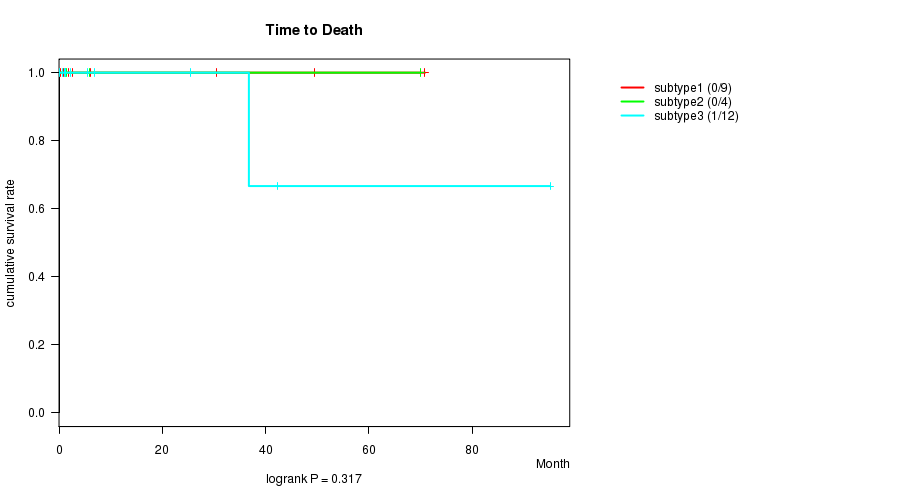
P value = 0.317 (logrank test)

Table S2. Clustering Approach #1: 'CN CNMF' versus Clinical Feature #1: 'Time to Death'

	nPatients	nDeath	Duration Range (Median), Month
ALL	25	1	0.1 - 95.1 (2.7)
subtype1	9	0	0.3 - 70.8 (2.7)
subtype2	4	0	1.2 - 69.9 (3.6)
subtype3	12	1	0.1 - 95.1 (3.8)

Figure S1. Get High-res Image Clustering Approach #1: 'CN CNMF' versus Clinical Feature #1: 'Time to Death'

'CN CNMF' versus 'AGE'

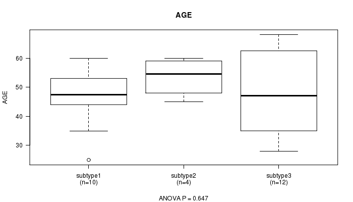
P value = 0.647 (ANOVA)

Table S3. Clustering Approach #1: 'CN CNMF' versus Clinical Feature #2: 'AGE'

	nPatients	Mean (Std.Dev)
ALL	26	48.5 (11.8)
subtype1	10	46.8 (10.4)
subtype2	4	53.5 (6.9)
subtype3	12	48.2 (14.3)

Figure S2. Get High-res Image Clustering Approach #1: 'CN CNMF' versus Clinical Feature #2: 'AGE'

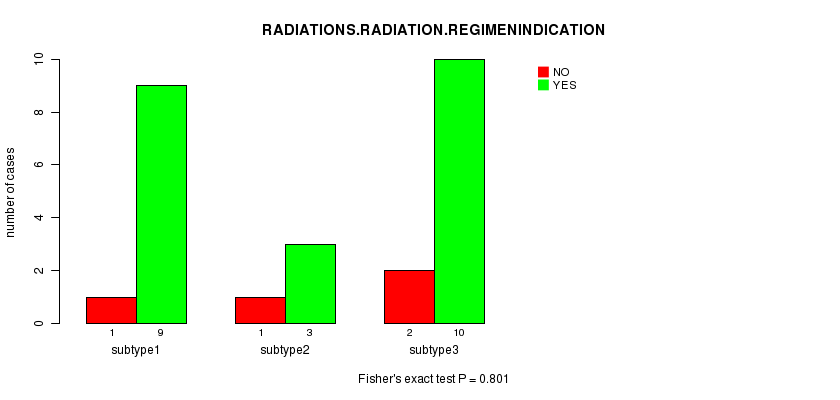
'CN CNMF' versus 'RADIATIONS.RADIATION.REGIMENINDICATION'

P value = 0.801 (Fisher's exact test)

Table S4. Clustering Approach #1: 'CN CNMF' versus Clinical Feature #3: 'RADIATIONS.RADIATION.REGIMENINDICATION'

nPatients	NO	YES
ALL	4	22
subtype1	1	9
subtype2	1	3
subtype3	2	10

Figure S3. Get High-res Image Clustering Approach #1: 'CN CNMF' versus Clinical Feature #3: 'RADIATIONS.RADIATION.REGIMENINDICATION'

'CN CNMF' versus 'NEOADJUVANT.THERAPY'

P value = 0.801 (Fisher's exact test)

Table S5. Clustering Approach #1: 'CN CNMF' versus Clinical Feature #4: 'NEOADJUVANT.THERAPY'

nPatients	NO	YES
ALL	4	22
subtype1	1	9
subtype2	1	3
subtype3	2	10

Figure S4. Get High-res Image Clustering Approach #1: 'CN CNMF' versus Clinical Feature #4: 'NEOADJUVANT.THERAPY'

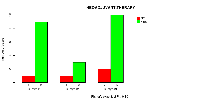
Clustering Approach #2: 'MIRseq CNMF subtypes'

Table S6. Get Full Table Description of clustering approach #2: 'MIRseq CNMF subtypes'

Cluster Labels	1	2	3
Number of samples	9	4	4

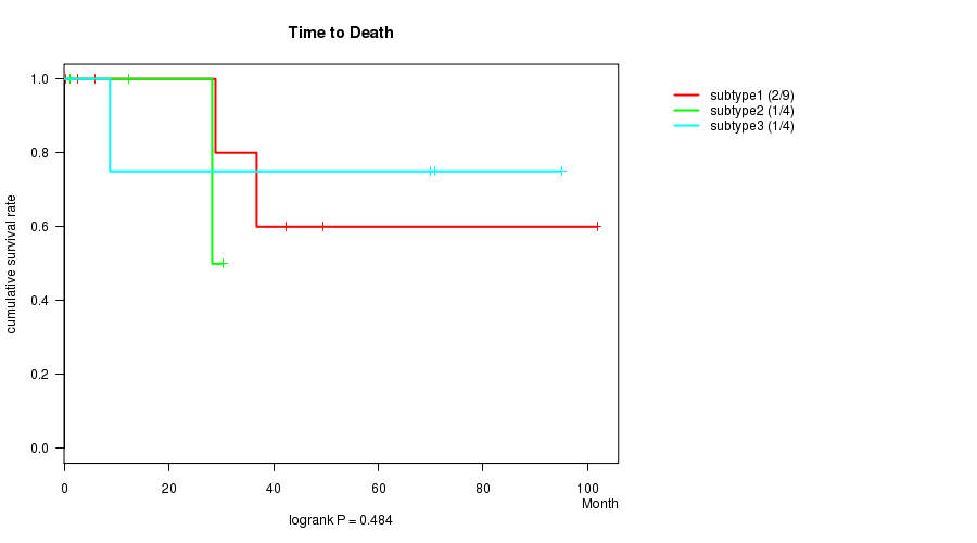
'MIRseq CNMF subtypes' versus 'Time to Death'

P value = 0.484 (logrank test)

Table S7. Clustering Approach #2: 'MIRseq CNMF subtypes' versus Clinical Feature #1: 'Time to Death'

	nPatients	nDeath	Duration Range (Median), Month
ALL	17	4	0.3 - 101.8 (28.9)
subtype1	9	2	0.3 - 101.8 (28.9)
subtype2	4	1	1.2 - 30.4 (20.3)
subtype3	4	1	8.8 - 95.1 (70.4)

Figure S5. Get High-res Image Clustering Approach #2: 'MIRseq CNMF subtypes' versus Clinical Feature #1: 'Time to Death'

'MIRseq CNMF subtypes' versus 'AGE'

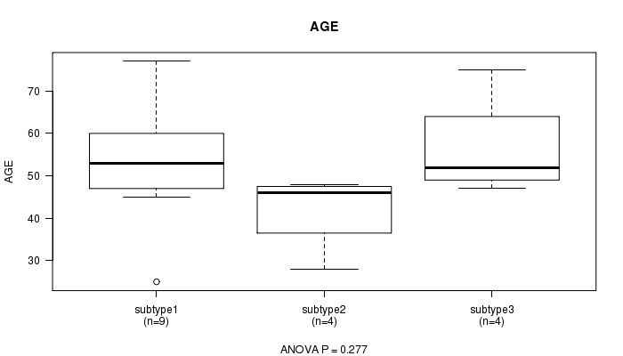
P value = 0.277 (ANOVA)

Table S8. Clustering Approach #2: 'MIRseq CNMF subtypes' versus Clinical Feature #2: 'AGE'

	nPatients	Mean (Std.Dev)
ALL	17	51.1 (13.3)
subtype1	9	52.8 (14.2)
subtype2	4	42.0 (9.4)
subtype3	4	56.5 (12.6)

Figure S6. Get High-res Image Clustering Approach #2: 'MIRseq CNMF subtypes' versus Clinical Feature #2: 'AGE'

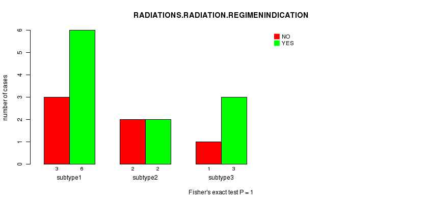
'MIRseq CNMF subtypes' versus 'RADIATIONS.RADIATION.REGIMENINDICATION'

P value = 1 (Fisher's exact test)

Table S9. Clustering Approach #2: 'MIRseq CNMF subtypes' versus Clinical Feature #3: 'RADIATIONS.RADIATION.REGIMENINDICATION'

nPatients	NO	YES
ALL	6	11
subtype1	3	6
subtype2	2	2
subtype3	1	3

Figure S7. Get High-res Image Clustering Approach #2: 'MIRseq CNMF subtypes' versus Clinical Feature #3: 'RADIATIONS.RADIATION.REGIMENINDICATION'

'MIRseq CNMF subtypes' versus 'NEOADJUVANT.THERAPY'

P value = 0.511 (Fisher's exact test)

Table S10. Clustering Approach #2: 'MIRseq CNMF subtypes' versus Clinical Feature #4: 'NEOADJUVANT.THERAPY'

nPatients	NO	YES
ALL	6	11
subtype1	2	7
subtype2	2	2
subtype3	2	2

Figure S8. Get High-res Image Clustering Approach #2: 'MIRseq CNMF subtypes' versus Clinical Feature #4: 'NEOADJUVANT.THERAPY'

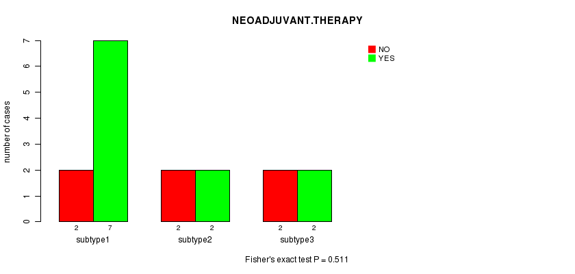
Clustering Approach #3: 'MIRseq cHierClus subtypes'

Table S11. Get Full Table Description of clustering approach #3: 'MIRseq cHierClus subtypes'

Cluster Labels	1	2	3	4	5
Number of samples	3	1	3	2	8

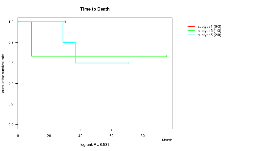
'MIRseq cHierClus subtypes' versus 'Time to Death'

P value = 0.531 (logrank test)

Table S12. Clustering Approach #3: 'MIRseq cHierClus subtypes' versus Clinical Feature #1: 'Time to Death'

	nPatients	nDeath	Duration Range (Median), Month
ALL	14	3	0.3 - 95.1 (29.7)
subtype1	3	0	1.2 - 30.4 (12.4)
subtype3	3	1	8.8 - 95.1 (69.9)
subtype5	8	2	0.3 - 70.8 (32.8)

Figure S9. Get High-res Image Clustering Approach #3: 'MIRseq cHierClus subtypes' versus Clinical Feature #1: 'Time to Death'

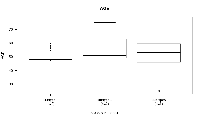
'MIRseq cHierClus subtypes' versus 'AGE'

P value = 0.831 (ANOVA)

Table S13. Clustering Approach #3: 'MIRseq cHierClus subtypes' versus Clinical Feature #2: 'AGE'

	nPatients	Mean (Std.Dev)
ALL	14	53.4 (13.0)
subtype1	3	51.7 (7.2)
subtype3	3	57.7 (15.1)
subtype5	8	52.4 (14.9)

Figure S10. Get High-res Image Clustering Approach #3: 'MIRseq cHierClus subtypes' versus Clinical Feature #2: 'AGE'

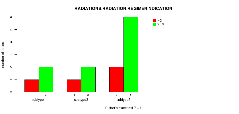
'MIRseq cHierClus subtypes' versus 'RADIATIONS.RADIATION.REGIMENINDICATION'

P value = 1 (Fisher's exact test)

Table S14. Clustering Approach #3: 'MIRseq cHierClus subtypes' versus Clinical Feature #3: 'RADIATIONS.RADIATION.REGIMENINDICATION'

nPatients	NO	YES
ALL	4	10
subtype1	1	2
subtype3	1	2
subtype5	2	6

Figure S11. Get High-res Image Clustering Approach #3: 'MIRseq cHierClus subtypes' versus Clinical Feature #3: 'RADIATIONS.RADIATION.REGIMENINDICATION'

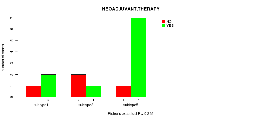
'MIRseq cHierClus subtypes' versus 'NEOADJUVANT.THERAPY'

P value = 0.245 (Fisher's exact test)

Table S15. Clustering Approach #3: 'MIRseq cHierClus subtypes' versus Clinical Feature #4: 'NEOADJUVANT.THERAPY'

nPatients	NO	YES
ALL	4	10
subtype1	1	2
subtype3	2	1
subtype5	1	7

Figure S12. Get High-res Image Clustering Approach #3: 'MIRseq cHierClus subtypes' versus Clinical Feature #4: 'NEOADJUVANT.THERAPY'

Methods & Data

Input

Cluster data file = CESC.mergedcluster.txt
Clinical data file = CESC.clin.merged.picked.txt
Number of patients = 31
Number of clustering approaches = 3
Number of selected clinical features = 4
Exclude small clusters that include fewer than K patients, K = 3

Clustering approaches

CNMF clustering

consensus non-negative matrix factorization clustering approach (Brunet et al. 2004)

Consensus hierarchical clustering

Resampling-based clustering method (Monti et al. 2003)

Survival analysis

For survival clinical features, the Kaplan-Meier survival curves of tumors with and without gene mutations were plotted and the statistical significance P values were estimated by logrank test (Bland and Altman 2004) using the 'survdiff' function in R

ANOVA analysis

For continuous numerical clinical features, one-way analysis of variance (Howell 2002) was applied to compare the clinical values between tumor subtypes using 'anova' function in R

Fisher's exact test

For binary clinical features, two-tailed Fisher's exact tests (Fisher 1922) were used to estimate the P values using the 'fisher.test' function in R

Download Results

This is an experimental feature. The full results of the analysis summarized in this report can be downloaded from the TCGA Data Coordination Center.

References

[1] Brunet et al., Metagenes and molecular pattern discovery using matrix factorization, PNAS 101(12):4164-9 (2004)

[2] Monti et al., Consensus Clustering: A Resampling-Based Method for Class Discovery and Visualization of Gene Expression Microarray Data, Machine Learning 52(1):91-118 (2003)

[3] Bland and Altman, Statistics notes: The logrank test, BMJ 328(7447):1073 (2004)

[4] Howell, D, Statistical Methods for Psychology. (5th ed.), Duxbury Press:324-5 (2002)

[5] Fisher, R.A., On the interpretation of chi-square from contingency tables, and the calculation of P, Journal of the Royal Statistical Society 85(1):87-94 (1922)

Made with Nozzle