Kidney Renal Clear Cell Carcinoma: Correlation between gene mutation status and selected clinical features<BR>(primary solid tumor cohort)

Kidney Renal Clear Cell Carcinoma: Correlation between gene mutation status and selected clinical features
(primary solid tumor cohort)

Maintained by TCGA GDAC Team (Broad Institute/MD Anderson Cancer Center/Harvard Medical School)

Overview

Introduction

This pipeline computes the correlation between significantly recurrent gene mutations and selected clinical features.

Summary

Testing the association between mutation status of 31 genes and 8 clinical features across 293 patients, 2 significant findings detected with Q value < 0.25.

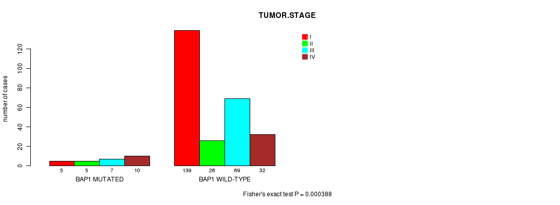
BAP1 mutation correlated to 'TUMOR.STAGE'.
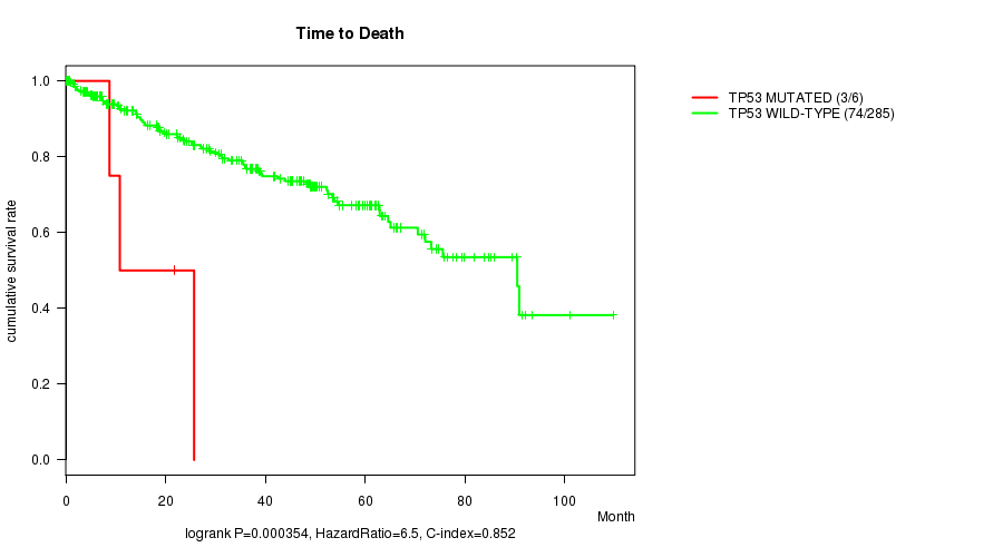
TP53 mutation correlated to 'Time to Death'.

Results

Overview of the results

Table 1. Get Full Table Overview of the association between mutation status of 31 genes and 8 clinical features. Shown in the table are P values (Q values). Thresholded by Q value < 0.25, 2 significant findings detected.


		Clinical Features	Time to Death	AGE	GENDER	KARNOFSKY PERFORMANCE SCORE	PATHOLOGY T	PATHOLOGY N	PATHOLOGICSPREAD(M)	TUMOR STAGE
	nMutated (%)	nWild-Type	logrank test	t-test	Fisher's exact test	t-test	Fisher's exact test	Fisher's exact test	Fisher's exact test	Fisher's exact test
BAP1	27 (9%)	266	0.0136 (1.00)	0.742 (1.00)	0.00238 (0.511)		0.00295 (0.63)	0.627 (1.00)	0.00411 (0.876)	0.000388 (0.0846)
TP53	6 (2%)	287	0.000354 (0.0775)	0.259 (1.00)	0.188 (1.00)		0.0158 (1.00)	0.271 (1.00)	0.579 (1.00)	0.0249 (1.00)
PBRM1	106 (36%)	187	0.525 (1.00)	0.892 (1.00)	0.16 (1.00)	0.429 (1.00)	0.86 (1.00)	0.746 (1.00)	0.592 (1.00)	0.901 (1.00)
VHL	138 (47%)	155	0.668 (1.00)	0.0301 (1.00)	0.269 (1.00)	0.359 (1.00)	0.0815 (1.00)	0.756 (1.00)	1 (1.00)	0.169 (1.00)
SETD2	33 (11%)	260	0.747 (1.00)	0.136 (1.00)	0.119 (1.00)		0.192 (1.00)	0.605 (1.00)	0.059 (1.00)	0.0967 (1.00)
KDM5C	18 (6%)	275	0.0803 (1.00)	0.206 (1.00)	0.00486 (1.00)		0.622 (1.00)	0.516 (1.00)	1 (1.00)	0.856 (1.00)
MUC4	41 (14%)	252	0.454 (1.00)	0.247 (1.00)	0.597 (1.00)		0.00706 (1.00)	0.217 (1.00)	0.0431 (1.00)	0.0021 (0.453)
MTOR	24 (8%)	269	0.123 (1.00)	0.203 (1.00)	0.119 (1.00)		0.298 (1.00)	0.0602 (1.00)	1 (1.00)	0.346 (1.00)
PTEN	9 (3%)	284	0.769 (1.00)	0.219 (1.00)	0.503 (1.00)		0.347 (1.00)	0.0286 (1.00)	0.613 (1.00)	0.0971 (1.00)
EBPL	6 (2%)	287	0.48 (1.00)	0.527 (1.00)	0.00161 (0.35)		0.117 (1.00)	1 (1.00)	1 (1.00)	0.0646 (1.00)
NBPF10	19 (6%)	274	0.173 (1.00)	0.305 (1.00)	0.133 (1.00)		0.147 (1.00)	0.113 (1.00)	0.0274 (1.00)	0.115 (1.00)
BAGE2	4 (1%)	289	0.961 (1.00)	0.667 (1.00)	0.612 (1.00)		0.796 (1.00)	1 (1.00)	1 (1.00)	0.589 (1.00)
PIK3CA	10 (3%)	283	0.253 (1.00)	0.808 (1.00)	0.743 (1.00)		0.342 (1.00)	1 (1.00)	1 (1.00)	0.336 (1.00)
WDR52	9 (3%)	284	0.967 (1.00)	0.395 (1.00)	0.724 (1.00)		0.647 (1.00)	1 (1.00)	0.342 (1.00)	0.842 (1.00)
TPTE2	7 (2%)	286	0.3 (1.00)	0.309 (1.00)	1 (1.00)		0.48 (1.00)	1 (1.00)	0.599 (1.00)	0.596 (1.00)
TSPAN19	4 (1%)	289	0.319 (1.00)	0.467 (1.00)	1 (1.00)		0.458 (1.00)	1 (1.00)	0.437 (1.00)	0.223 (1.00)
ANKRD7	4 (1%)	289	0.193 (1.00)	0.758 (1.00)	0.612 (1.00)		0.19 (1.00)	1 (1.00)	1 (1.00)	0.464 (1.00)
C5ORF13	3 (1%)	290	0.32 (1.00)	0.465 (1.00)	0.278 (1.00)		1 (1.00)	1 (1.00)	1 (1.00)	1 (1.00)
CNTNAP4	9 (3%)	284	0.485 (1.00)	0.5 (1.00)	0.724 (1.00)		0.51 (1.00)	1 (1.00)	1 (1.00)	0.513 (1.00)
CR1	10 (3%)	283	0.594 (1.00)	0.711 (1.00)	0.743 (1.00)		0.902 (1.00)	1 (1.00)	0.628 (1.00)	0.777 (1.00)
GFRAL	5 (2%)	288	0.655 (1.00)	0.0399 (1.00)	1 (1.00)		0.096 (1.00)	1 (1.00)	1 (1.00)	0.288 (1.00)
GRIN2B	11 (4%)	282	0.952 (1.00)	0.755 (1.00)	1 (1.00)		0.831 (1.00)	1 (1.00)	1 (1.00)	0.587 (1.00)
OR10G7	5 (2%)	288	0.0498 (1.00)	0.301 (1.00)	1 (1.00)		0.568 (1.00)	1 (1.00)	0.513 (1.00)	0.0542 (1.00)
SFRS15	9 (3%)	284	0.564 (1.00)	0.804 (1.00)	0.724 (1.00)		0.647 (1.00)	1 (1.00)	1 (1.00)	0.459 (1.00)
STAG2	9 (3%)	284	0.971 (1.00)	0.0169 (1.00)	1 (1.00)		0.112 (1.00)	1 (1.00)	1 (1.00)	0.161 (1.00)
CCNB2	5 (2%)	288	0.784 (1.00)	0.459 (1.00)	1 (1.00)		1 (1.00)	1 (1.00)	1 (1.00)	0.911 (1.00)
NPNT	6 (2%)	287	0.0806 (1.00)	0.222 (1.00)	0.668 (1.00)		0.342 (1.00)	1 (1.00)	1 (1.00)	0.219 (1.00)
LIPI	5 (2%)	288	0.507 (1.00)	0.0842 (1.00)	0.661 (1.00)		0.325 (1.00)	1 (1.00)	0.133 (1.00)	0.153 (1.00)
PCLO	20 (7%)	273	0.537 (1.00)	0.775 (1.00)	0.223 (1.00)		0.763 (1.00)	1 (1.00)	0.737 (1.00)	0.68 (1.00)
ZNF800	6 (2%)	287	0.166 (1.00)	0.599 (1.00)	1 (1.00)		1 (1.00)	1 (1.00)	0.579 (1.00)	0.806 (1.00)
SPAM1	5 (2%)	288	0.27 (1.00)	0.192 (1.00)	0.661 (1.00)		0.096 (1.00)	1 (1.00)	1 (1.00)	0.288 (1.00)

'BAP1 MUTATION STATUS' versus 'TUMOR.STAGE'

P value = 0.000388 (Fisher's exact test), Q value = 0.085

Table S1. Gene #3: 'BAP1 MUTATION STATUS' versus Clinical Feature #8: 'TUMOR.STAGE'

nPatients	I	II	III	IV
ALL	144	31	76	42
BAP1 MUTATED	5	5	7	10
BAP1 WILD-TYPE	139	26	69	32

Figure S1. Get High-res Image Gene #3: 'BAP1 MUTATION STATUS' versus Clinical Feature #8: 'TUMOR.STAGE'

'TP53 MUTATION STATUS' versus 'Time to Death'

P value = 0.000354 (logrank test), Q value = 0.077

Table S2. Gene #15: 'TP53 MUTATION STATUS' versus Clinical Feature #1: 'Time to Death'

	nPatients	nDeath	Duration Range (Median), Month
ALL	291	77	0.1 - 109.6 (34.3)
TP53 MUTATED	6	3	0.2 - 25.7 (9.8)
TP53 WILD-TYPE	285	74	0.1 - 109.6 (35.2)

Figure S2. Get High-res Image Gene #15: 'TP53 MUTATION STATUS' versus Clinical Feature #1: 'Time to Death'

Methods & Data

Input

Mutation data file = KIRC-TP.mutsig.cluster.txt
Clinical data file = KIRC-TP.clin.merged.picked.txt
Number of patients = 293
Number of significantly mutated genes = 31
Number of selected clinical features = 8
Exclude genes that fewer than K tumors have mutations, K = 3

Survival analysis

For survival clinical features, the Kaplan-Meier survival curves of tumors with and without gene mutations were plotted and the statistical significance P values were estimated by logrank test (Bland and Altman 2004) using the 'survdiff' function in R

Student's t-test analysis

For continuous numerical clinical features, two-tailed Student's t test with unequal variance (Lehmann and Romano 2005) was applied to compare the clinical values between tumors with and without gene mutations using 't.test' function in R

Fisher's exact test

For binary or multi-class clinical features (nominal or ordinal), two-tailed Fisher's exact tests (Fisher 1922) were used to estimate the P values using the 'fisher.test' function in R

Q value calculation

For multiple hypothesis correction, Q value is the False Discovery Rate (FDR) analogue of the P value (Benjamini and Hochberg 1995), defined as the minimum FDR at which the test may be called significant. We used the 'Benjamini and Hochberg' method of 'p.adjust' function in R to convert P values into Q values.

Download Results

This is an experimental feature. The full results of the analysis summarized in this report can be downloaded from the TCGA Data Coordination Center.

References

[1] Bland and Altman, Statistics notes: The logrank test, BMJ 328(7447):1073 (2004)

[2] Lehmann and Romano, Testing Statistical Hypotheses (3E ed.), New York: Springer. ISBN 0387988645 (2005)

[3] Fisher, R.A., On the interpretation of chi-square from contingency tables, and the calculation of P, Journal of the Royal Statistical Society 85(1):87-94 (1922)

[4] Benjamini and Hochberg, Controlling the false discovery rate: a practical and powerful approach to multiple testing, Journal of the Royal Statistical Society Series B 59:289-300 (1995)

Made with Nozzle