Correlation between copy number variations of arm-level result and selected clinical features

Prostate Adenocarcinoma (Primary solid tumor)

21 April 2013 | analyses__2013_04_21

Maintainer Information

Citation Information

Maintained by TCGA GDAC Team (Broad Institute/MD Anderson Cancer Center/Harvard Medical School)

Cite as Broad Institute TCGA Genome Data Analysis Center (2013): Prostate Adenocarcinoma (Primary solid tumor cohort) - 21 April 2013: Correlation between copy number variations of arm-level result and selected clinical features. Broad Institute of MIT and Harvard. doi:10.7908/C1JD4TRG

Overview

Introduction

This pipeline computes the correlation between significant arm-level copy number variations (cnvs) and selected clinical features.

Summary

Testing the association between copy number variation 25 arm-level results and 5 clinical features across 154 patients, 4 significant findings detected with Q value < 0.25.

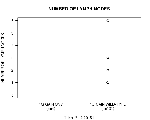
1q gain cnv correlated to 'NUMBER.OF.LYMPH.NODES'.
3p gain cnv correlated to 'NUMBER.OF.LYMPH.NODES'.
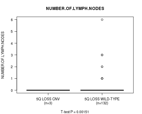
5q loss cnv correlated to 'NUMBER.OF.LYMPH.NODES'.
20p loss cnv correlated to 'NUMBER.OF.LYMPH.NODES'.

Results

Overview of the results

Table 1. Get Full Table Overview of the association between significant copy number variation of 25 arm-level results and 5 clinical features. Shown in the table are P values (Q values). Thresholded by Q value < 0.25, 4 significant findings detected.


		Clinical Features	Time to Death	AGE	RADIATIONS RADIATION REGIMENINDICATION	COMPLETENESS OF RESECTION	NUMBER OF LYMPH NODES
	nCNV (%)	nWild-Type	logrank test	t-test	Fisher's exact test	Fisher's exact test	t-test
1q gain	0 (0%)	150	1 (1.00)	0.302 (1.00)	1 (1.00)	0.228 (1.00)	0.00151 (0.187)
3p gain	0 (0%)	150	1 (1.00)	0.648 (1.00)	1 (1.00)	0.604 (1.00)	0.00151 (0.187)
5q loss	0 (0%)	151	1 (1.00)	0.217 (1.00)	1 (1.00)	1 (1.00)	0.00151 (0.187)
20p loss	0 (0%)	150	1 (1.00)	0.455 (1.00)	0.125 (1.00)	0.228 (1.00)	0.00151 (0.187)
3q gain	0 (0%)	149	1 (1.00)	0.362 (1.00)	1 (1.00)	1 (1.00)	0.439 (1.00)
7p gain	0 (0%)	140	1 (1.00)	0.0192 (1.00)	1 (1.00)	0.774 (1.00)	0.17 (1.00)
7q gain	0 (0%)	142	1 (1.00)	0.0695 (1.00)	1 (1.00)	1 (1.00)	0.958 (1.00)
8p gain	0 (0%)	147	1 (1.00)	0.636 (1.00)	1 (1.00)	0.405 (1.00)	0.685 (1.00)
8q gain	0 (0%)	140	1 (1.00)	0.694 (1.00)	1 (1.00)	0.427 (1.00)	0.856 (1.00)
9p gain	0 (0%)	151	1 (1.00)	0.725 (1.00)	1 (1.00)		0.555 (1.00)
9q gain	0 (0%)	150	1 (1.00)	0.7 (1.00)	1 (1.00)	1 (1.00)	0.555 (1.00)
10q gain	0 (0%)	151	1 (1.00)	0.146 (1.00)	1 (1.00)	1 (1.00)	0.456 (1.00)
6q loss	0 (0%)	147	1 (1.00)	0.261 (1.00)	1 (1.00)	1 (1.00)	0.609 (1.00)
8p loss	0 (0%)	115	1 (1.00)	0.0895 (1.00)	0.331 (1.00)	0.495 (1.00)	0.0935 (1.00)
8q loss	0 (0%)	150	1 (1.00)	0.651 (1.00)	1 (1.00)	1 (1.00)	0.248 (1.00)
10p loss	0 (0%)	150	1 (1.00)	0.674 (1.00)	1 (1.00)	1 (1.00)	0.875 (1.00)
10q loss	0 (0%)	150	1 (1.00)	0.395 (1.00)	1 (1.00)	0.604 (1.00)	0.328 (1.00)
12p loss	0 (0%)	147	1 (1.00)	0.671 (1.00)	1 (1.00)	0.405 (1.00)	0.142 (1.00)
13q loss	0 (0%)	143	1 (1.00)	0.819 (1.00)	1 (1.00)	1 (1.00)	0.1 (1.00)
16q loss	0 (0%)	134	1 (1.00)	0.286 (1.00)	1 (1.00)	0.638 (1.00)	0.207 (1.00)
17p loss	0 (0%)	135	1 (1.00)	0.464 (1.00)	1 (1.00)	0.517 (1.00)	0.129 (1.00)
18p loss	0 (0%)	140	1 (1.00)	0.861 (1.00)	1 (1.00)	0.544 (1.00)	0.487 (1.00)
18q loss	0 (0%)	134	1 (1.00)	0.72 (1.00)	1 (1.00)	0.517 (1.00)	0.242 (1.00)
21q loss	0 (0%)	151	1 (1.00)	0.405 (1.00)	1 (1.00)	1 (1.00)	0.503 (1.00)
22q loss	0 (0%)	150	1 (1.00)	0.467 (1.00)	0.125 (1.00)	0.228 (1.00)	0.511 (1.00)

'1q gain' versus 'NUMBER.OF.LYMPH.NODES'

P value = 0.00151 (t-test), Q value = 0.19

Table S1. Gene #1: '1q gain' versus Clinical Feature #5: 'NUMBER.OF.LYMPH.NODES'

	nPatients	Mean (Std.Dev)
ALL	135	0.2 (0.7)
1Q GAIN CNV	4	0.0 (0.0)
1Q GAIN WILD-TYPE	131	0.2 (0.8)

Figure S1. Get High-res Image Gene #1: '1q gain' versus Clinical Feature #5: 'NUMBER.OF.LYMPH.NODES'

'3p gain' versus 'NUMBER.OF.LYMPH.NODES'

P value = 0.00151 (t-test), Q value = 0.19

Table S2. Gene #2: '3p gain' versus Clinical Feature #5: 'NUMBER.OF.LYMPH.NODES'

	nPatients	Mean (Std.Dev)
ALL	135	0.2 (0.7)
3P GAIN CNV	4	0.0 (0.0)
3P GAIN WILD-TYPE	131	0.2 (0.8)

Figure S2. Get High-res Image Gene #2: '3p gain' versus Clinical Feature #5: 'NUMBER.OF.LYMPH.NODES'

'5q loss' versus 'NUMBER.OF.LYMPH.NODES'

P value = 0.00151 (t-test), Q value = 0.19

Table S3. Gene #11: '5q loss' versus Clinical Feature #5: 'NUMBER.OF.LYMPH.NODES'

	nPatients	Mean (Std.Dev)
ALL	135	0.2 (0.7)
5Q LOSS CNV	3	0.0 (0.0)
5Q LOSS WILD-TYPE	132	0.2 (0.8)

Figure S3. Get High-res Image Gene #11: '5q loss' versus Clinical Feature #5: 'NUMBER.OF.LYMPH.NODES'

'20p loss' versus 'NUMBER.OF.LYMPH.NODES'

P value = 0.00151 (t-test), Q value = 0.19

Table S4. Gene #23: '20p loss' versus Clinical Feature #5: 'NUMBER.OF.LYMPH.NODES'

	nPatients	Mean (Std.Dev)
ALL	135	0.2 (0.7)
20P LOSS CNV	4	0.0 (0.0)
20P LOSS WILD-TYPE	131	0.2 (0.8)

Figure S4. Get High-res Image Gene #23: '20p loss' versus Clinical Feature #5: 'NUMBER.OF.LYMPH.NODES'

Methods & Data

Input

Mutation data file = broad_values_by_arm.mutsig.cluster.txt
Clinical data file = PRAD-TP.clin.merged.picked.txt
Number of patients = 154
Number of significantly arm-level cnvs = 25
Number of selected clinical features = 5
Exclude genes that fewer than K tumors have mutations, K = 3

Survival analysis

For survival clinical features, the Kaplan-Meier survival curves of tumors with and without gene mutations were plotted and the statistical significance P values were estimated by logrank test (Bland and Altman 2004) using the 'survdiff' function in R

Student's t-test analysis

For continuous numerical clinical features, two-tailed Student's t test with unequal variance (Lehmann and Romano 2005) was applied to compare the clinical values between tumors with and without gene mutations using 't.test' function in R

Fisher's exact test

For binary or multi-class clinical features (nominal or ordinal), two-tailed Fisher's exact tests (Fisher 1922) were used to estimate the P values using the 'fisher.test' function in R

Q value calculation

For multiple hypothesis correction, Q value is the False Discovery Rate (FDR) analogue of the P value (Benjamini and Hochberg 1995), defined as the minimum FDR at which the test may be called significant. We used the 'Benjamini and Hochberg' method of 'p.adjust' function in R to convert P values into Q values.

Download Results

This is an experimental feature. The full results of the analysis summarized in this report can be downloaded from the TCGA Data Coordination Center.

References

[1] Bland and Altman, Statistics notes: The logrank test, BMJ 328(7447):1073 (2004)

[2] Lehmann and Romano, Testing Statistical Hypotheses (3E ed.), New York: Springer. ISBN 0387988645 (2005)

[3] Fisher, R.A., On the interpretation of chi-square from contingency tables, and the calculation of P, Journal of the Royal Statistical Society 85(1):87-94 (1922)

[4] Benjamini and Hochberg, Controlling the false discovery rate: a practical and powerful approach to multiple testing, Journal of the Royal Statistical Society Series B 59:289-300 (1995)

Made with Nozzle