This pipeline computes the correlation between cancer subtypes identified by different molecular patterns and selected clinical features.
Testing the association between subtypes identified by 6 different clustering approaches and 7 clinical features across 22 patients, 4 significant findings detected with P value < 0.05 and Q value < 0.25.
-
3 subtypes identified in current cancer cohort by 'Copy Number Ratio CNMF subtypes'. These subtypes correlate to 'AGE'.
-
3 subtypes identified in current cancer cohort by 'METHLYATION CNMF'. These subtypes do not correlate to any clinical features.
-
3 subtypes identified in current cancer cohort by 'MIRSEQ CNMF'. These subtypes do not correlate to any clinical features.
-
2 subtypes identified in current cancer cohort by 'MIRSEQ CHIERARCHICAL'. These subtypes correlate to 'AGE'.
-
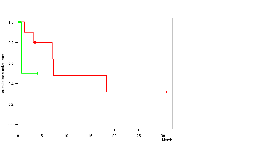
3 subtypes identified in current cancer cohort by 'MIRseq Mature CNMF subtypes'. These subtypes correlate to 'Time to Death'.
-
2 subtypes identified in current cancer cohort by 'MIRseq Mature cHierClus subtypes'. These subtypes correlate to 'AGE'.
Table 1. Get Full Table Overview of the association between subtypes identified by 6 different clustering approaches and 7 clinical features. Shown in the table are P values (Q values). Thresholded by P value < 0.05 and Q value < 0.25, 4 significant findings detected.
|
Clinical Features |
Statistical Tests |
Copy Number Ratio CNMF subtypes |
METHLYATION CNMF |
MIRSEQ CNMF |
MIRSEQ CHIERARCHICAL |
MIRseq Mature CNMF subtypes |
MIRseq Mature cHierClus subtypes |
| Time to Death | logrank test |
0.583 (1.00) |
0.819 (1.00) |
0.25 (1.00) |
0.25 (1.00) |
0.0027 (0.111) |
0.25 (1.00) |
| AGE | t-test |
0.00199 (0.0837) |
0.178 (1.00) |
0.0122 (0.464) |
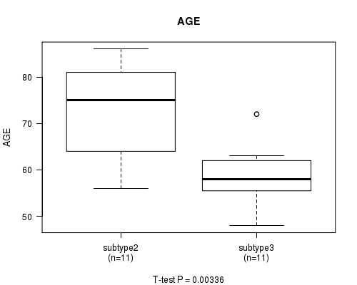
0.00336 (0.134) |
0.0183 (0.675) |
0.00336 (0.134) |
| NEOPLASM DISEASESTAGE | Chi-square test |
0.359 (1.00) |
0.307 (1.00) |
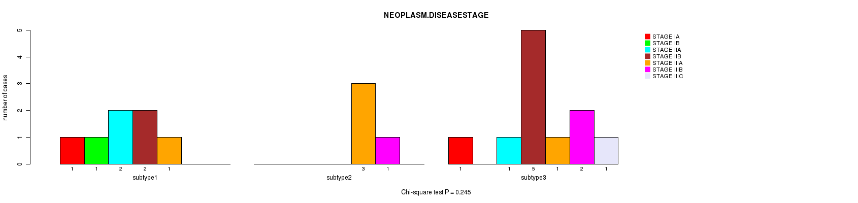
0.245 (1.00) |
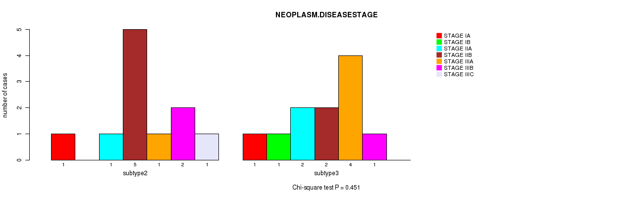
0.451 (1.00) |
0.0638 (1.00) |
0.451 (1.00) |
| PATHOLOGY T STAGE | Chi-square test |
0.422 (1.00) |
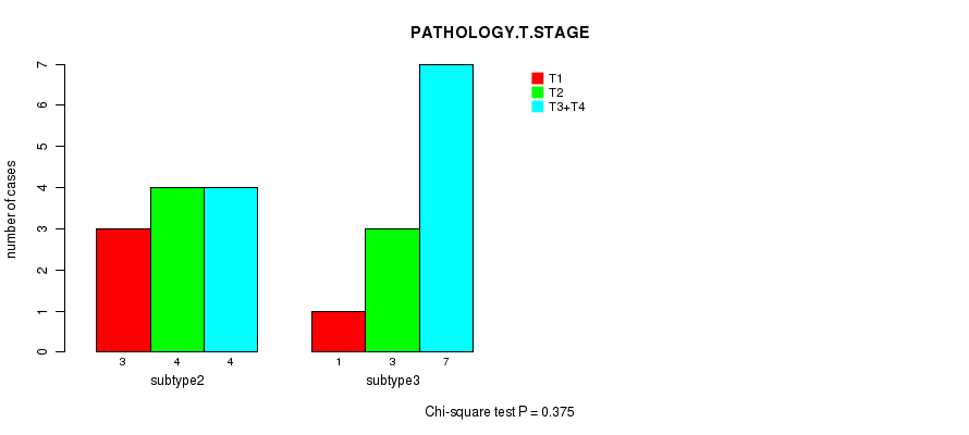
0.375 (1.00) |
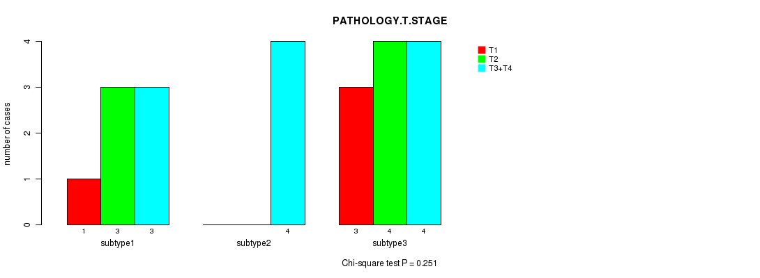
0.251 (1.00) |
0.375 (1.00) |
0.217 (1.00) |
0.375 (1.00) |
| PATHOLOGY N STAGE | Chi-square test |
0.122 (1.00) |
0.872 (1.00) |
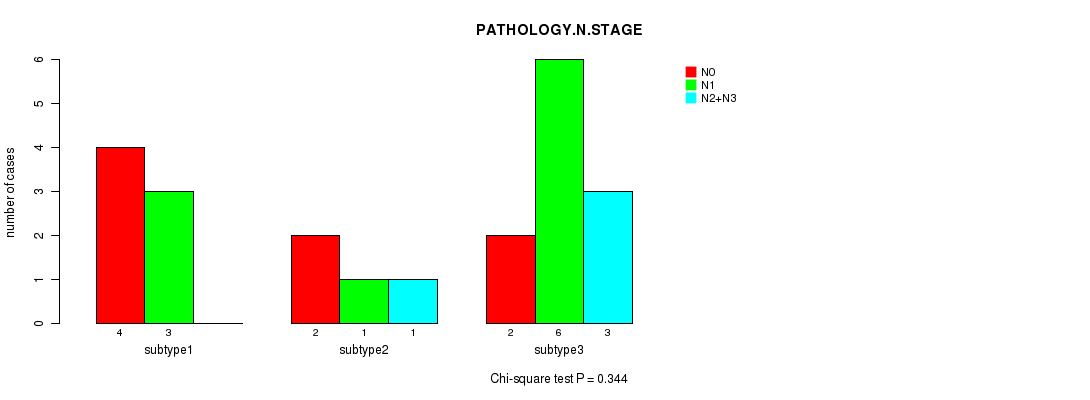
0.344 (1.00) |
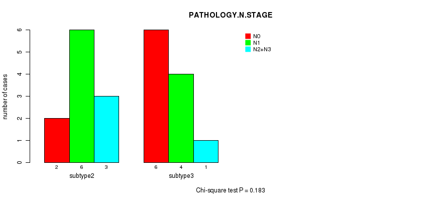
0.183 (1.00) |
0.578 (1.00) |
0.183 (1.00) |
| GENDER | Fisher's exact test |
1 (1.00) |
1 (1.00) |
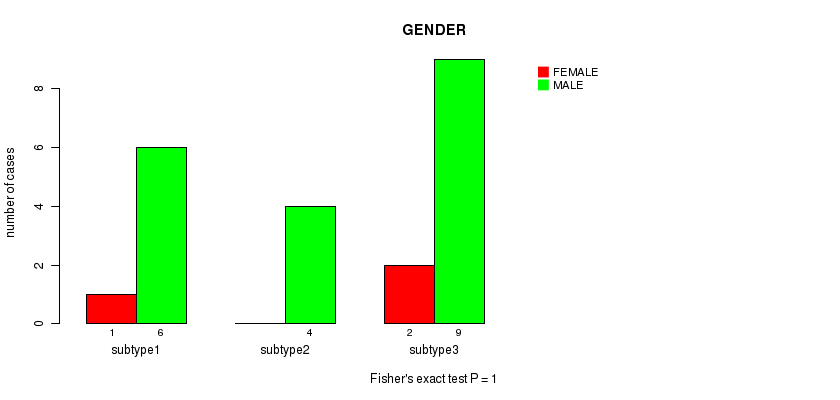
1 (1.00) |
1 (1.00) |
0.684 (1.00) |
1 (1.00) |
| NUMBERPACKYEARSSMOKED | t-test |
0.588 (1.00) |
0.882 (1.00) |
0.381 (1.00) |
0.187 (1.00) |
0.5 (1.00) |
0.187 (1.00) |
Table S1. Description of clustering approach #1: 'Copy Number Ratio CNMF subtypes'
| Cluster Labels | 1 | 2 | 3 |
|---|---|---|---|
| Number of samples | 3 | 12 | 7 |
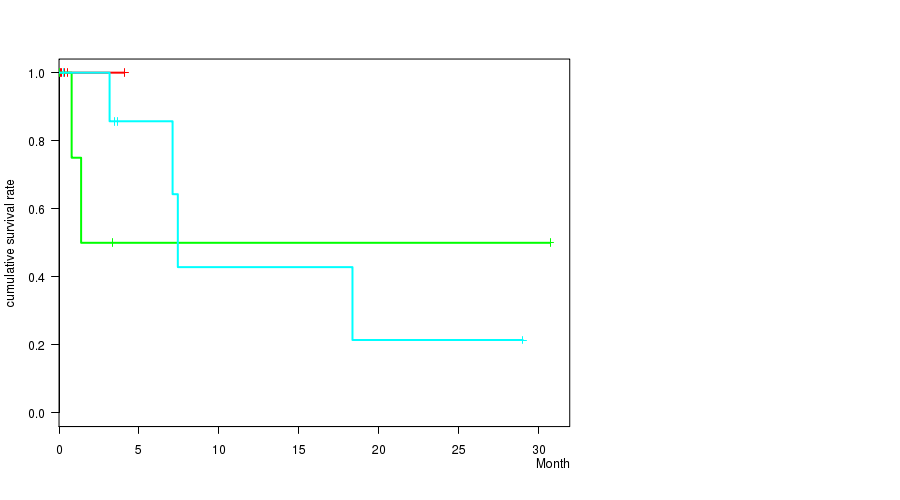
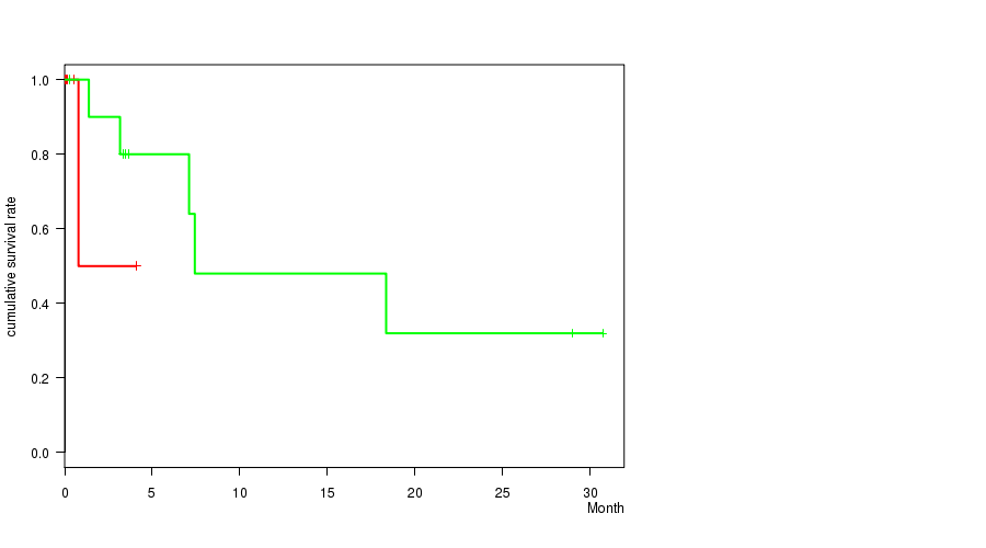
P value = 0.583 (logrank test), Q value = 1
Table S2. Clustering Approach #1: 'Copy Number Ratio CNMF subtypes' versus Clinical Feature #1: 'Time to Death'
| nPatients | nDeath | Duration Range (Median), Month | |
|---|---|---|---|
| ALL | 18 | 6 | 0.0 - 30.7 (3.2) |
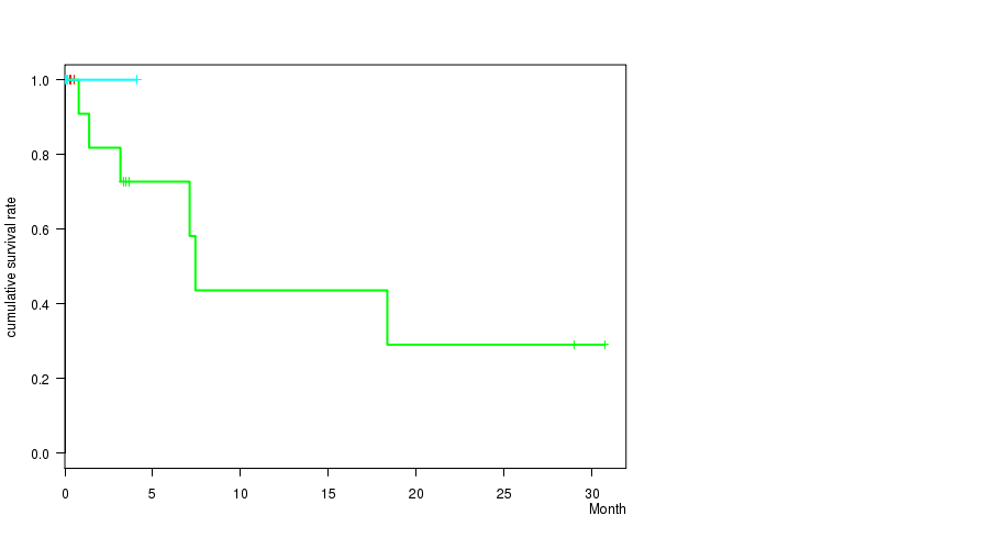
| subtype1 | 3 | 0 | 0.3 - 0.5 (0.4) |
| subtype2 | 11 | 6 | 0.8 - 30.7 (3.7) |
| subtype3 | 4 | 0 | 0.0 - 4.1 (0.1) |
Figure S1. Get High-res Image Clustering Approach #1: 'Copy Number Ratio CNMF subtypes' versus Clinical Feature #1: 'Time to Death'
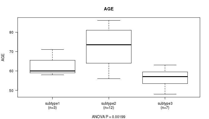
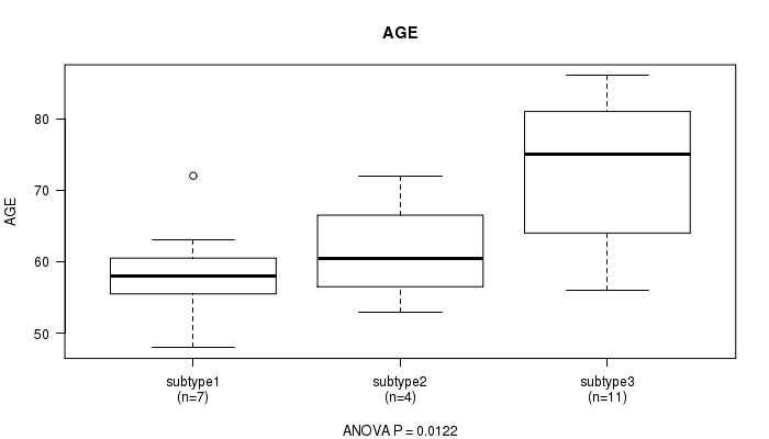
P value = 0.00199 (ANOVA), Q value = 0.084
Table S3. Clustering Approach #1: 'Copy Number Ratio CNMF subtypes' versus Clinical Feature #2: 'AGE'
| nPatients | Mean (Std.Dev) | |
|---|---|---|
| ALL | 22 | 66.0 (10.8) |
| subtype1 | 3 | 63.0 (7.0) |
| subtype2 | 12 | 72.4 (9.7) |
| subtype3 | 7 | 56.3 (5.1) |
Figure S2. Get High-res Image Clustering Approach #1: 'Copy Number Ratio CNMF subtypes' versus Clinical Feature #2: 'AGE'
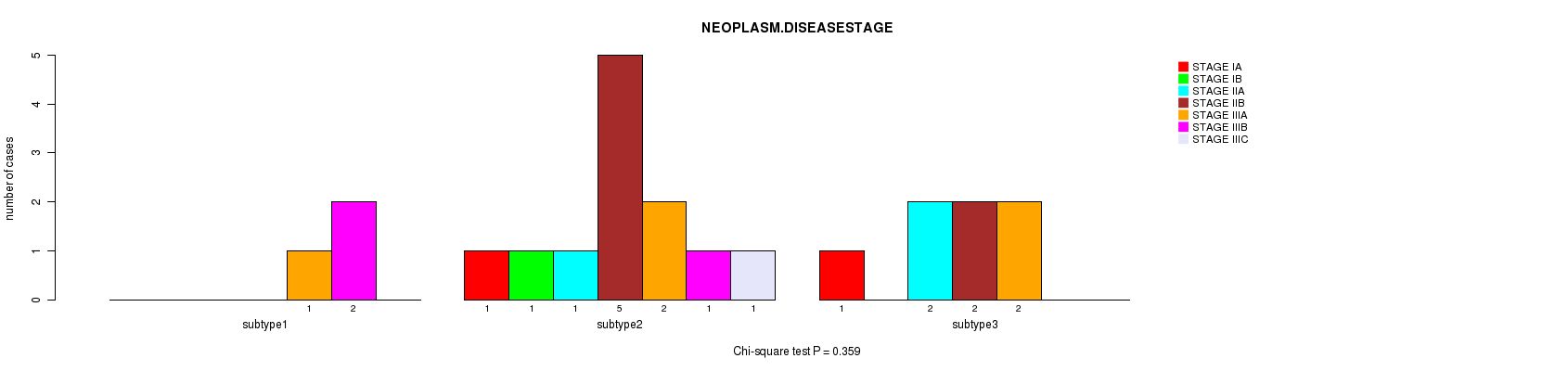
P value = 0.359 (Chi-square test), Q value = 1
Table S4. Clustering Approach #1: 'Copy Number Ratio CNMF subtypes' versus Clinical Feature #3: 'NEOPLASM.DISEASESTAGE'
| nPatients | STAGE IA | STAGE IB | STAGE IIA | STAGE IIB | STAGE IIIA | STAGE IIIB | STAGE IIIC |
|---|---|---|---|---|---|---|---|
| ALL | 2 | 1 | 3 | 7 | 5 | 3 | 1 |
| subtype1 | 0 | 0 | 0 | 0 | 1 | 2 | 0 |
| subtype2 | 1 | 1 | 1 | 5 | 2 | 1 | 1 |
| subtype3 | 1 | 0 | 2 | 2 | 2 | 0 | 0 |
Figure S3. Get High-res Image Clustering Approach #1: 'Copy Number Ratio CNMF subtypes' versus Clinical Feature #3: 'NEOPLASM.DISEASESTAGE'
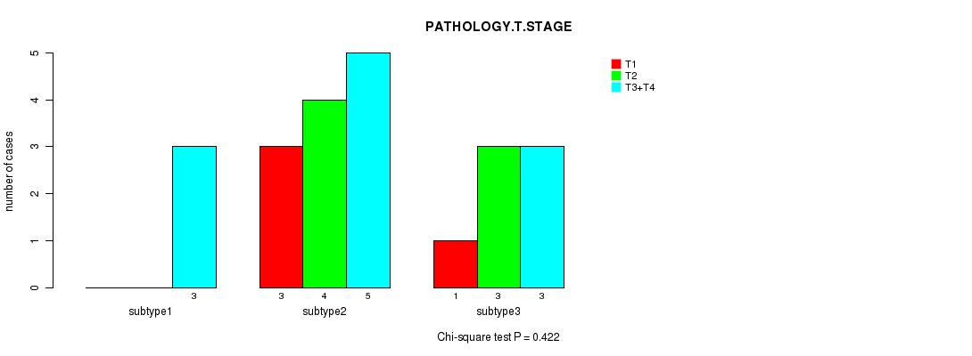
P value = 0.422 (Chi-square test), Q value = 1
Table S5. Clustering Approach #1: 'Copy Number Ratio CNMF subtypes' versus Clinical Feature #4: 'PATHOLOGY.T.STAGE'
| nPatients | T1 | T2 | T3+T4 |
|---|---|---|---|
| ALL | 4 | 7 | 11 |
| subtype1 | 0 | 0 | 3 |
| subtype2 | 3 | 4 | 5 |
| subtype3 | 1 | 3 | 3 |
Figure S4. Get High-res Image Clustering Approach #1: 'Copy Number Ratio CNMF subtypes' versus Clinical Feature #4: 'PATHOLOGY.T.STAGE'
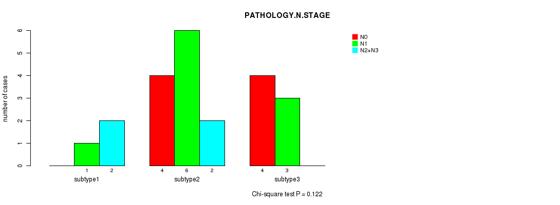
P value = 0.122 (Chi-square test), Q value = 1
Table S6. Clustering Approach #1: 'Copy Number Ratio CNMF subtypes' versus Clinical Feature #5: 'PATHOLOGY.N.STAGE'
| nPatients | N0 | N1 | N2+N3 |
|---|---|---|---|
| ALL | 8 | 10 | 4 |
| subtype1 | 0 | 1 | 2 |
| subtype2 | 4 | 6 | 2 |
| subtype3 | 4 | 3 | 0 |
Figure S5. Get High-res Image Clustering Approach #1: 'Copy Number Ratio CNMF subtypes' versus Clinical Feature #5: 'PATHOLOGY.N.STAGE'
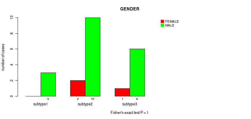
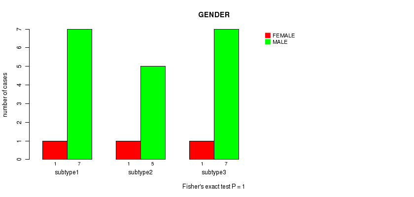
P value = 1 (Fisher's exact test), Q value = 1
Table S7. Clustering Approach #1: 'Copy Number Ratio CNMF subtypes' versus Clinical Feature #6: 'GENDER'
| nPatients | FEMALE | MALE |
|---|---|---|
| ALL | 3 | 19 |
| subtype1 | 0 | 3 |
| subtype2 | 2 | 10 |
| subtype3 | 1 | 6 |
Figure S6. Get High-res Image Clustering Approach #1: 'Copy Number Ratio CNMF subtypes' versus Clinical Feature #6: 'GENDER'
P value = 0.588 (ANOVA), Q value = 1
Table S8. Clustering Approach #1: 'Copy Number Ratio CNMF subtypes' versus Clinical Feature #7: 'NUMBERPACKYEARSSMOKED'
| nPatients | Mean (Std.Dev) | |
|---|---|---|
| ALL | 14 | 32.7 (17.6) |
| subtype1 | 1 | 31.0 (NA) |
| subtype2 | 9 | 34.4 (21.2) |
| subtype3 | 4 | 29.4 (10.9) |
Figure S7. Get High-res Image Clustering Approach #1: 'Copy Number Ratio CNMF subtypes' versus Clinical Feature #7: 'NUMBERPACKYEARSSMOKED'
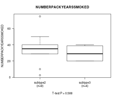
Table S9. Description of clustering approach #2: 'METHLYATION CNMF'
| Cluster Labels | 1 | 2 | 3 |
|---|---|---|---|
| Number of samples | 8 | 6 | 8 |
P value = 0.819 (logrank test), Q value = 1
Table S10. Clustering Approach #2: 'METHLYATION CNMF' versus Clinical Feature #1: 'Time to Death'
| nPatients | nDeath | Duration Range (Median), Month | |
|---|---|---|---|
| ALL | 18 | 6 | 0.0 - 30.7 (3.2) |
| subtype1 | 5 | 0 | 0.1 - 4.1 (0.4) |
| subtype2 | 5 | 2 | 0.0 - 30.7 (1.4) |
| subtype3 | 8 | 4 | 0.3 - 29.0 (5.4) |
Figure S8. Get High-res Image Clustering Approach #2: 'METHLYATION CNMF' versus Clinical Feature #1: 'Time to Death'
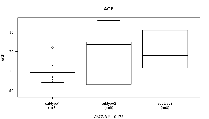
P value = 0.178 (ANOVA), Q value = 1
Table S11. Clustering Approach #2: 'METHLYATION CNMF' versus Clinical Feature #2: 'AGE'
| nPatients | Mean (Std.Dev) | |
|---|---|---|
| ALL | 22 | 66.0 (10.8) |
| subtype1 | 8 | 60.4 (5.4) |
| subtype2 | 6 | 68.2 (14.6) |
| subtype3 | 8 | 70.0 (10.6) |
Figure S9. Get High-res Image Clustering Approach #2: 'METHLYATION CNMF' versus Clinical Feature #2: 'AGE'
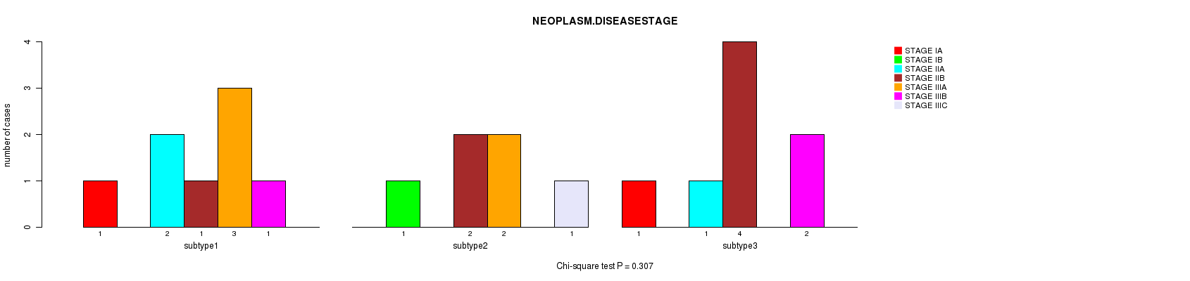
P value = 0.307 (Chi-square test), Q value = 1
Table S12. Clustering Approach #2: 'METHLYATION CNMF' versus Clinical Feature #3: 'NEOPLASM.DISEASESTAGE'
| nPatients | STAGE IA | STAGE IB | STAGE IIA | STAGE IIB | STAGE IIIA | STAGE IIIB | STAGE IIIC |
|---|---|---|---|---|---|---|---|
| ALL | 2 | 1 | 3 | 7 | 5 | 3 | 1 |
| subtype1 | 1 | 0 | 2 | 1 | 3 | 1 | 0 |
| subtype2 | 0 | 1 | 0 | 2 | 2 | 0 | 1 |
| subtype3 | 1 | 0 | 1 | 4 | 0 | 2 | 0 |
Figure S10. Get High-res Image Clustering Approach #2: 'METHLYATION CNMF' versus Clinical Feature #3: 'NEOPLASM.DISEASESTAGE'
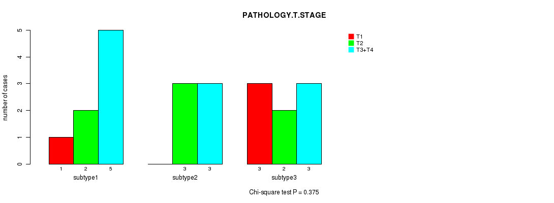
P value = 0.375 (Chi-square test), Q value = 1
Table S13. Clustering Approach #2: 'METHLYATION CNMF' versus Clinical Feature #4: 'PATHOLOGY.T.STAGE'
| nPatients | T1 | T2 | T3+T4 |
|---|---|---|---|
| ALL | 4 | 7 | 11 |
| subtype1 | 1 | 2 | 5 |
| subtype2 | 0 | 3 | 3 |
| subtype3 | 3 | 2 | 3 |
Figure S11. Get High-res Image Clustering Approach #2: 'METHLYATION CNMF' versus Clinical Feature #4: 'PATHOLOGY.T.STAGE'
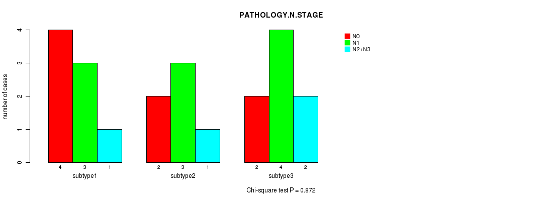
P value = 0.872 (Chi-square test), Q value = 1
Table S14. Clustering Approach #2: 'METHLYATION CNMF' versus Clinical Feature #5: 'PATHOLOGY.N.STAGE'
| nPatients | N0 | N1 | N2+N3 |
|---|---|---|---|
| ALL | 8 | 10 | 4 |
| subtype1 | 4 | 3 | 1 |
| subtype2 | 2 | 3 | 1 |
| subtype3 | 2 | 4 | 2 |
Figure S12. Get High-res Image Clustering Approach #2: 'METHLYATION CNMF' versus Clinical Feature #5: 'PATHOLOGY.N.STAGE'
P value = 1 (Fisher's exact test), Q value = 1
Table S15. Clustering Approach #2: 'METHLYATION CNMF' versus Clinical Feature #6: 'GENDER'
| nPatients | FEMALE | MALE |
|---|---|---|
| ALL | 3 | 19 |
| subtype1 | 1 | 7 |
| subtype2 | 1 | 5 |
| subtype3 | 1 | 7 |
Figure S13. Get High-res Image Clustering Approach #2: 'METHLYATION CNMF' versus Clinical Feature #6: 'GENDER'
P value = 0.882 (ANOVA), Q value = 1
Table S16. Clustering Approach #2: 'METHLYATION CNMF' versus Clinical Feature #7: 'NUMBERPACKYEARSSMOKED'
| nPatients | Mean (Std.Dev) | |
|---|---|---|
| ALL | 14 | 32.7 (17.6) |
| subtype1 | 4 | 35.2 (12.8) |
| subtype2 | 5 | 34.0 (26.8) |
| subtype3 | 5 | 29.4 (11.9) |
Figure S14. Get High-res Image Clustering Approach #2: 'METHLYATION CNMF' versus Clinical Feature #7: 'NUMBERPACKYEARSSMOKED'
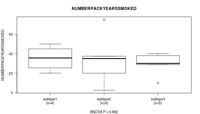
Table S17. Description of clustering approach #3: 'MIRSEQ CNMF'
| Cluster Labels | 1 | 2 | 3 |
|---|---|---|---|
| Number of samples | 7 | 4 | 11 |
P value = 0.25 (logrank test), Q value = 1
Table S18. Clustering Approach #3: 'MIRSEQ CNMF' versus Clinical Feature #1: 'Time to Death'
| nPatients | nDeath | Duration Range (Median), Month | |
|---|---|---|---|
| ALL | 18 | 6 | 0.0 - 30.7 (3.2) |
| subtype1 | 6 | 1 | 0.0 - 4.1 (0.3) |
| subtype2 | 1 | 0 | 0.4 - 0.4 (0.4) |
| subtype3 | 11 | 5 | 0.3 - 30.7 (3.7) |
Figure S15. Get High-res Image Clustering Approach #3: 'MIRSEQ CNMF' versus Clinical Feature #1: 'Time to Death'
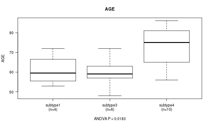
P value = 0.0122 (ANOVA), Q value = 0.46
Table S19. Clustering Approach #3: 'MIRSEQ CNMF' versus Clinical Feature #2: 'AGE'
| nPatients | Mean (Std.Dev) | |
|---|---|---|
| ALL | 22 | 66.0 (10.8) |
| subtype1 | 7 | 58.6 (7.5) |
| subtype2 | 4 | 61.5 (7.9) |
| subtype3 | 11 | 72.4 (10.1) |
Figure S16. Get High-res Image Clustering Approach #3: 'MIRSEQ CNMF' versus Clinical Feature #2: 'AGE'
P value = 0.245 (Chi-square test), Q value = 1
Table S20. Clustering Approach #3: 'MIRSEQ CNMF' versus Clinical Feature #3: 'NEOPLASM.DISEASESTAGE'
| nPatients | STAGE IA | STAGE IB | STAGE IIA | STAGE IIB | STAGE IIIA | STAGE IIIB | STAGE IIIC |
|---|---|---|---|---|---|---|---|
| ALL | 2 | 1 | 3 | 7 | 5 | 3 | 1 |
| subtype1 | 1 | 1 | 2 | 2 | 1 | 0 | 0 |
| subtype2 | 0 | 0 | 0 | 0 | 3 | 1 | 0 |
| subtype3 | 1 | 0 | 1 | 5 | 1 | 2 | 1 |
Figure S17. Get High-res Image Clustering Approach #3: 'MIRSEQ CNMF' versus Clinical Feature #3: 'NEOPLASM.DISEASESTAGE'
P value = 0.251 (Chi-square test), Q value = 1
Table S21. Clustering Approach #3: 'MIRSEQ CNMF' versus Clinical Feature #4: 'PATHOLOGY.T.STAGE'
| nPatients | T1 | T2 | T3+T4 |
|---|---|---|---|
| ALL | 4 | 7 | 11 |
| subtype1 | 1 | 3 | 3 |
| subtype2 | 0 | 0 | 4 |
| subtype3 | 3 | 4 | 4 |
Figure S18. Get High-res Image Clustering Approach #3: 'MIRSEQ CNMF' versus Clinical Feature #4: 'PATHOLOGY.T.STAGE'
P value = 0.344 (Chi-square test), Q value = 1
Table S22. Clustering Approach #3: 'MIRSEQ CNMF' versus Clinical Feature #5: 'PATHOLOGY.N.STAGE'
| nPatients | N0 | N1 | N2+N3 |
|---|---|---|---|
| ALL | 8 | 10 | 4 |
| subtype1 | 4 | 3 | 0 |
| subtype2 | 2 | 1 | 1 |
| subtype3 | 2 | 6 | 3 |
Figure S19. Get High-res Image Clustering Approach #3: 'MIRSEQ CNMF' versus Clinical Feature #5: 'PATHOLOGY.N.STAGE'
P value = 1 (Fisher's exact test), Q value = 1
Table S23. Clustering Approach #3: 'MIRSEQ CNMF' versus Clinical Feature #6: 'GENDER'
| nPatients | FEMALE | MALE |
|---|---|---|
| ALL | 3 | 19 |
| subtype1 | 1 | 6 |
| subtype2 | 0 | 4 |
| subtype3 | 2 | 9 |
Figure S20. Get High-res Image Clustering Approach #3: 'MIRSEQ CNMF' versus Clinical Feature #6: 'GENDER'
P value = 0.381 (ANOVA), Q value = 1
Table S24. Clustering Approach #3: 'MIRSEQ CNMF' versus Clinical Feature #7: 'NUMBERPACKYEARSSMOKED'
| nPatients | Mean (Std.Dev) | |
|---|---|---|
| ALL | 14 | 32.7 (17.6) |
| subtype1 | 5 | 37.2 (22.7) |
| subtype2 | 2 | 43.8 (8.8) |
| subtype3 | 7 | 26.3 (14.4) |
Figure S21. Get High-res Image Clustering Approach #3: 'MIRSEQ CNMF' versus Clinical Feature #7: 'NUMBERPACKYEARSSMOKED'
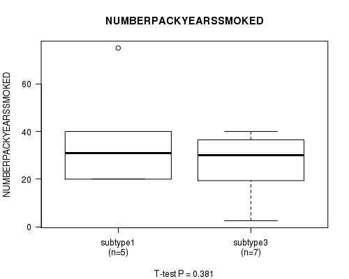
Table S25. Description of clustering approach #4: 'MIRSEQ CHIERARCHICAL'
| Cluster Labels | 2 | 3 |
|---|---|---|
| Number of samples | 11 | 11 |
P value = 0.25 (logrank test), Q value = 1
Table S26. Clustering Approach #4: 'MIRSEQ CHIERARCHICAL' versus Clinical Feature #1: 'Time to Death'
| nPatients | nDeath | Duration Range (Median), Month | |
|---|---|---|---|
| ALL | 18 | 6 | 0.0 - 30.7 (3.2) |
| subtype2 | 11 | 5 | 0.3 - 30.7 (3.7) |
| subtype3 | 7 | 1 | 0.0 - 4.1 (0.4) |
Figure S22. Get High-res Image Clustering Approach #4: 'MIRSEQ CHIERARCHICAL' versus Clinical Feature #1: 'Time to Death'

P value = 0.00336 (t-test), Q value = 0.13
Table S27. Clustering Approach #4: 'MIRSEQ CHIERARCHICAL' versus Clinical Feature #2: 'AGE'
| nPatients | Mean (Std.Dev) | |
|---|---|---|
| ALL | 22 | 66.0 (10.8) |
| subtype2 | 11 | 72.4 (10.1) |
| subtype3 | 11 | 59.6 (7.4) |
Figure S23. Get High-res Image Clustering Approach #4: 'MIRSEQ CHIERARCHICAL' versus Clinical Feature #2: 'AGE'
P value = 0.451 (Chi-square test), Q value = 1
Table S28. Clustering Approach #4: 'MIRSEQ CHIERARCHICAL' versus Clinical Feature #3: 'NEOPLASM.DISEASESTAGE'
| nPatients | STAGE IA | STAGE IB | STAGE IIA | STAGE IIB | STAGE IIIA | STAGE IIIB | STAGE IIIC |
|---|---|---|---|---|---|---|---|
| ALL | 2 | 1 | 3 | 7 | 5 | 3 | 1 |
| subtype2 | 1 | 0 | 1 | 5 | 1 | 2 | 1 |
| subtype3 | 1 | 1 | 2 | 2 | 4 | 1 | 0 |
Figure S24. Get High-res Image Clustering Approach #4: 'MIRSEQ CHIERARCHICAL' versus Clinical Feature #3: 'NEOPLASM.DISEASESTAGE'
P value = 0.375 (Chi-square test), Q value = 1
Table S29. Clustering Approach #4: 'MIRSEQ CHIERARCHICAL' versus Clinical Feature #4: 'PATHOLOGY.T.STAGE'
| nPatients | T1 | T2 | T3+T4 |
|---|---|---|---|
| ALL | 4 | 7 | 11 |
| subtype2 | 3 | 4 | 4 |
| subtype3 | 1 | 3 | 7 |
Figure S25. Get High-res Image Clustering Approach #4: 'MIRSEQ CHIERARCHICAL' versus Clinical Feature #4: 'PATHOLOGY.T.STAGE'

P value = 0.183 (Chi-square test), Q value = 1
Table S30. Clustering Approach #4: 'MIRSEQ CHIERARCHICAL' versus Clinical Feature #5: 'PATHOLOGY.N.STAGE'
| nPatients | N0 | N1 | N2+N3 |
|---|---|---|---|
| ALL | 8 | 10 | 4 |
| subtype2 | 2 | 6 | 3 |
| subtype3 | 6 | 4 | 1 |
Figure S26. Get High-res Image Clustering Approach #4: 'MIRSEQ CHIERARCHICAL' versus Clinical Feature #5: 'PATHOLOGY.N.STAGE'

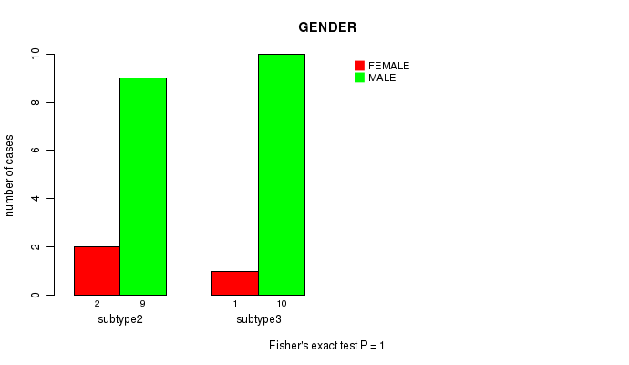
P value = 1 (Fisher's exact test), Q value = 1
Table S31. Clustering Approach #4: 'MIRSEQ CHIERARCHICAL' versus Clinical Feature #6: 'GENDER'
| nPatients | FEMALE | MALE |
|---|---|---|
| ALL | 3 | 19 |
| subtype2 | 2 | 9 |
| subtype3 | 1 | 10 |
Figure S27. Get High-res Image Clustering Approach #4: 'MIRSEQ CHIERARCHICAL' versus Clinical Feature #6: 'GENDER'
P value = 0.187 (t-test), Q value = 1
Table S32. Clustering Approach #4: 'MIRSEQ CHIERARCHICAL' versus Clinical Feature #7: 'NUMBERPACKYEARSSMOKED'
| nPatients | Mean (Std.Dev) | |
|---|---|---|
| ALL | 14 | 32.7 (17.6) |
| subtype2 | 7 | 26.3 (14.4) |
| subtype3 | 7 | 39.1 (19.2) |
Figure S28. Get High-res Image Clustering Approach #4: 'MIRSEQ CHIERARCHICAL' versus Clinical Feature #7: 'NUMBERPACKYEARSSMOKED'
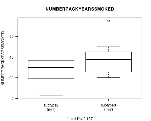
Table S33. Description of clustering approach #5: 'MIRseq Mature CNMF subtypes'
| Cluster Labels | 1 | 2 | 3 | 4 |
|---|---|---|---|---|
| Number of samples | 4 | 2 | 6 | 10 |
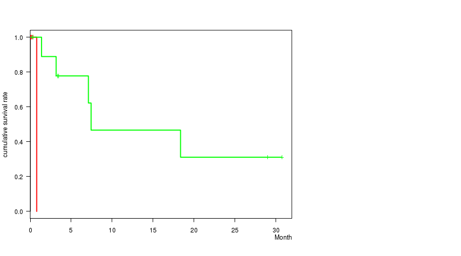
P value = 0.0027 (logrank test), Q value = 0.11
Table S34. Clustering Approach #5: 'MIRseq Mature CNMF subtypes' versus Clinical Feature #1: 'Time to Death'
| nPatients | nDeath | Duration Range (Median), Month | |
|---|---|---|---|
| ALL | 16 | 6 | 0.0 - 30.7 (2.3) |
| subtype1 | 1 | 0 | 0.5 - 0.5 (0.5) |
| subtype3 | 5 | 1 | 0.0 - 0.8 (0.1) |
| subtype4 | 10 | 5 | 0.3 - 30.7 (5.3) |
Figure S29. Get High-res Image Clustering Approach #5: 'MIRseq Mature CNMF subtypes' versus Clinical Feature #1: 'Time to Death'
P value = 0.0183 (ANOVA), Q value = 0.68
Table S35. Clustering Approach #5: 'MIRseq Mature CNMF subtypes' versus Clinical Feature #2: 'AGE'
| nPatients | Mean (Std.Dev) | |
|---|---|---|
| ALL | 20 | 66.8 (11.0) |
| subtype1 | 4 | 61.0 (8.0) |
| subtype3 | 6 | 59.7 (7.9) |
| subtype4 | 10 | 73.3 (10.2) |
Figure S30. Get High-res Image Clustering Approach #5: 'MIRseq Mature CNMF subtypes' versus Clinical Feature #2: 'AGE'
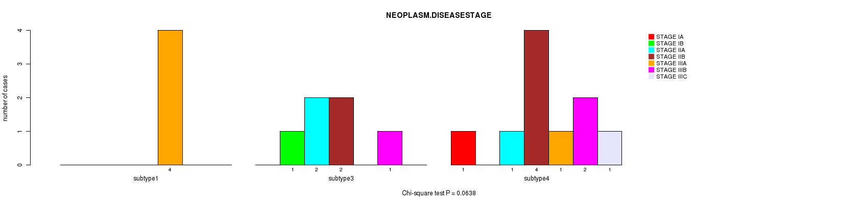
P value = 0.0638 (Chi-square test), Q value = 1
Table S36. Clustering Approach #5: 'MIRseq Mature CNMF subtypes' versus Clinical Feature #3: 'NEOPLASM.DISEASESTAGE'
| nPatients | STAGE IA | STAGE IB | STAGE IIA | STAGE IIB | STAGE IIIA | STAGE IIIB | STAGE IIIC |
|---|---|---|---|---|---|---|---|
| ALL | 1 | 1 | 3 | 6 | 5 | 3 | 1 |
| subtype1 | 0 | 0 | 0 | 0 | 4 | 0 | 0 |
| subtype3 | 0 | 1 | 2 | 2 | 0 | 1 | 0 |
| subtype4 | 1 | 0 | 1 | 4 | 1 | 2 | 1 |
Figure S31. Get High-res Image Clustering Approach #5: 'MIRseq Mature CNMF subtypes' versus Clinical Feature #3: 'NEOPLASM.DISEASESTAGE'
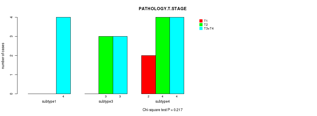
P value = 0.217 (Chi-square test), Q value = 1
Table S37. Clustering Approach #5: 'MIRseq Mature CNMF subtypes' versus Clinical Feature #4: 'PATHOLOGY.T.STAGE'
| nPatients | T1 | T2 | T3+T4 |
|---|---|---|---|
| ALL | 2 | 7 | 11 |
| subtype1 | 0 | 0 | 4 |
| subtype3 | 0 | 3 | 3 |
| subtype4 | 2 | 4 | 4 |
Figure S32. Get High-res Image Clustering Approach #5: 'MIRseq Mature CNMF subtypes' versus Clinical Feature #4: 'PATHOLOGY.T.STAGE'
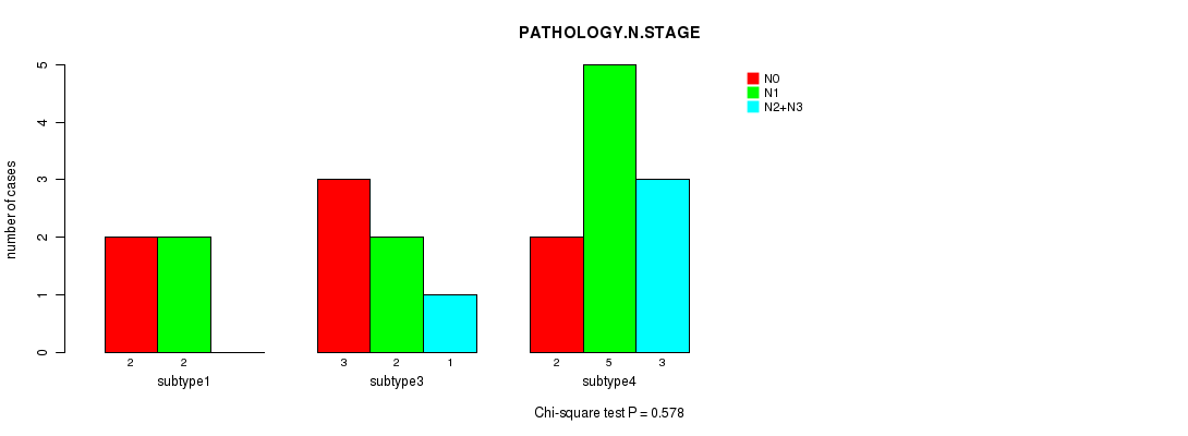
P value = 0.578 (Chi-square test), Q value = 1
Table S38. Clustering Approach #5: 'MIRseq Mature CNMF subtypes' versus Clinical Feature #5: 'PATHOLOGY.N.STAGE'
| nPatients | N0 | N1 | N2+N3 |
|---|---|---|---|
| ALL | 7 | 9 | 4 |
| subtype1 | 2 | 2 | 0 |
| subtype3 | 3 | 2 | 1 |
| subtype4 | 2 | 5 | 3 |
Figure S33. Get High-res Image Clustering Approach #5: 'MIRseq Mature CNMF subtypes' versus Clinical Feature #5: 'PATHOLOGY.N.STAGE'
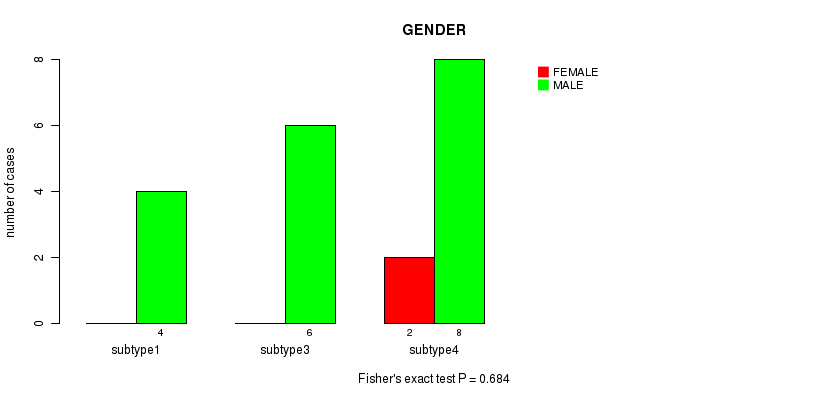
P value = 0.684 (Fisher's exact test), Q value = 1
Table S39. Clustering Approach #5: 'MIRseq Mature CNMF subtypes' versus Clinical Feature #6: 'GENDER'
| nPatients | FEMALE | MALE |
|---|---|---|
| ALL | 2 | 18 |
| subtype1 | 0 | 4 |
| subtype3 | 0 | 6 |
| subtype4 | 2 | 8 |
Figure S34. Get High-res Image Clustering Approach #5: 'MIRseq Mature CNMF subtypes' versus Clinical Feature #6: 'GENDER'
P value = 0.5 (ANOVA), Q value = 1
Table S40. Clustering Approach #5: 'MIRseq Mature CNMF subtypes' versus Clinical Feature #7: 'NUMBERPACKYEARSSMOKED'
| nPatients | Mean (Std.Dev) | |
|---|---|---|
| ALL | 13 | 32.1 (18.2) |
| subtype1 | 3 | 39.5 (9.7) |
| subtype3 | 3 | 38.3 (31.8) |
| subtype4 | 7 | 26.3 (14.4) |
Figure S35. Get High-res Image Clustering Approach #5: 'MIRseq Mature CNMF subtypes' versus Clinical Feature #7: 'NUMBERPACKYEARSSMOKED'
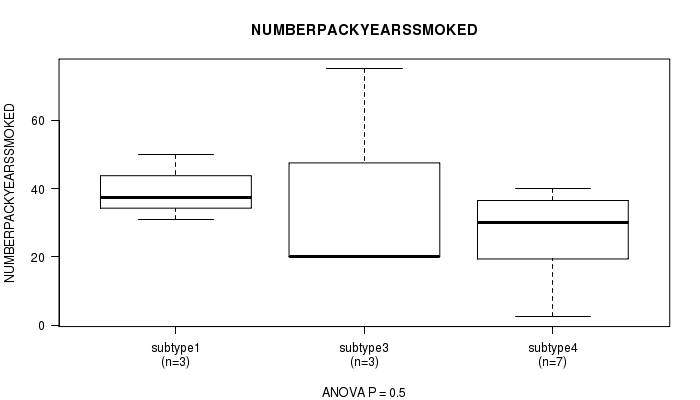
Table S41. Description of clustering approach #6: 'MIRseq Mature cHierClus subtypes'
| Cluster Labels | 2 | 3 |
|---|---|---|
| Number of samples | 11 | 11 |
P value = 0.25 (logrank test), Q value = 1
Table S42. Clustering Approach #6: 'MIRseq Mature cHierClus subtypes' versus Clinical Feature #1: 'Time to Death'
| nPatients | nDeath | Duration Range (Median), Month | |
|---|---|---|---|
| ALL | 18 | 6 | 0.0 - 30.7 (3.2) |
| subtype2 | 11 | 5 | 0.3 - 30.7 (3.7) |
| subtype3 | 7 | 1 | 0.0 - 4.1 (0.4) |
Figure S36. Get High-res Image Clustering Approach #6: 'MIRseq Mature cHierClus subtypes' versus Clinical Feature #1: 'Time to Death'
P value = 0.00336 (t-test), Q value = 0.13
Table S43. Clustering Approach #6: 'MIRseq Mature cHierClus subtypes' versus Clinical Feature #2: 'AGE'
| nPatients | Mean (Std.Dev) | |
|---|---|---|
| ALL | 22 | 66.0 (10.8) |
| subtype2 | 11 | 72.4 (10.1) |
| subtype3 | 11 | 59.6 (7.4) |
Figure S37. Get High-res Image Clustering Approach #6: 'MIRseq Mature cHierClus subtypes' versus Clinical Feature #2: 'AGE'

P value = 0.451 (Chi-square test), Q value = 1
Table S44. Clustering Approach #6: 'MIRseq Mature cHierClus subtypes' versus Clinical Feature #3: 'NEOPLASM.DISEASESTAGE'
| nPatients | STAGE IA | STAGE IB | STAGE IIA | STAGE IIB | STAGE IIIA | STAGE IIIB | STAGE IIIC |
|---|---|---|---|---|---|---|---|
| ALL | 2 | 1 | 3 | 7 | 5 | 3 | 1 |
| subtype2 | 1 | 0 | 1 | 5 | 1 | 2 | 1 |
| subtype3 | 1 | 1 | 2 | 2 | 4 | 1 | 0 |
Figure S38. Get High-res Image Clustering Approach #6: 'MIRseq Mature cHierClus subtypes' versus Clinical Feature #3: 'NEOPLASM.DISEASESTAGE'

P value = 0.375 (Chi-square test), Q value = 1
Table S45. Clustering Approach #6: 'MIRseq Mature cHierClus subtypes' versus Clinical Feature #4: 'PATHOLOGY.T.STAGE'
| nPatients | T1 | T2 | T3+T4 |
|---|---|---|---|
| ALL | 4 | 7 | 11 |
| subtype2 | 3 | 4 | 4 |
| subtype3 | 1 | 3 | 7 |
Figure S39. Get High-res Image Clustering Approach #6: 'MIRseq Mature cHierClus subtypes' versus Clinical Feature #4: 'PATHOLOGY.T.STAGE'
P value = 0.183 (Chi-square test), Q value = 1
Table S46. Clustering Approach #6: 'MIRseq Mature cHierClus subtypes' versus Clinical Feature #5: 'PATHOLOGY.N.STAGE'
| nPatients | N0 | N1 | N2+N3 |
|---|---|---|---|
| ALL | 8 | 10 | 4 |
| subtype2 | 2 | 6 | 3 |
| subtype3 | 6 | 4 | 1 |
Figure S40. Get High-res Image Clustering Approach #6: 'MIRseq Mature cHierClus subtypes' versus Clinical Feature #5: 'PATHOLOGY.N.STAGE'
P value = 1 (Fisher's exact test), Q value = 1
Table S47. Clustering Approach #6: 'MIRseq Mature cHierClus subtypes' versus Clinical Feature #6: 'GENDER'
| nPatients | FEMALE | MALE |
|---|---|---|
| ALL | 3 | 19 |
| subtype2 | 2 | 9 |
| subtype3 | 1 | 10 |
Figure S41. Get High-res Image Clustering Approach #6: 'MIRseq Mature cHierClus subtypes' versus Clinical Feature #6: 'GENDER'

P value = 0.187 (t-test), Q value = 1
Table S48. Clustering Approach #6: 'MIRseq Mature cHierClus subtypes' versus Clinical Feature #7: 'NUMBERPACKYEARSSMOKED'
| nPatients | Mean (Std.Dev) | |
|---|---|---|
| ALL | 14 | 32.7 (17.6) |
| subtype2 | 7 | 26.3 (14.4) |
| subtype3 | 7 | 39.1 (19.2) |
Figure S42. Get High-res Image Clustering Approach #6: 'MIRseq Mature cHierClus subtypes' versus Clinical Feature #7: 'NUMBERPACKYEARSSMOKED'

-
Cluster data file = ESCA-TP.mergedcluster.txt
-
Clinical data file = ESCA-TP.merged_data.txt
-
Number of patients = 22
-
Number of clustering approaches = 6
-
Number of selected clinical features = 7
-
Exclude small clusters that include fewer than K patients, K = 3
For survival clinical features, the Kaplan-Meier survival curves of tumors with and without gene mutations were plotted and the statistical significance P values were estimated by logrank test (Bland and Altman 2004) using the 'survdiff' function in R
For continuous numerical clinical features, one-way analysis of variance (Howell 2002) was applied to compare the clinical values between tumor subtypes using 'anova' function in R
For multi-class clinical features (nominal or ordinal), Chi-square tests (Greenwood and Nikulin 1996) were used to estimate the P values using the 'chisq.test' function in R
For binary clinical features, two-tailed Fisher's exact tests (Fisher 1922) were used to estimate the P values using the 'fisher.test' function in R
For continuous numerical clinical features, two-tailed Student's t test with unequal variance (Lehmann and Romano 2005) was applied to compare the clinical values between two tumor subtypes using 't.test' function in R
For multiple hypothesis correction, Q value is the False Discovery Rate (FDR) analogue of the P value (Benjamini and Hochberg 1995), defined as the minimum FDR at which the test may be called significant. We used the 'Benjamini and Hochberg' method of 'p.adjust' function in R to convert P values into Q values.
In addition to the links below, the full results of the analysis summarized in this report can also be downloaded programmatically using firehose_get, or interactively from either the Broad GDAC website or TCGA Data Coordination Center Portal.