Correlation between aggregated molecular cancer subtypes and selected clinical features

Prostate Adenocarcinoma (Primary solid tumor)

17 October 2014 | analyses__2014_10_17

Maintainer Information

Citation Information

Maintained by TCGA GDAC Team (Broad Institute/MD Anderson Cancer Center/Harvard Medical School)

Cite as Broad Institute TCGA Genome Data Analysis Center (2014): Correlation between aggregated molecular cancer subtypes and selected clinical features. Broad Institute of MIT and Harvard. doi:10.7908/C16Q1W5J

Overview

Introduction

This pipeline computes the correlation between cancer subtypes identified by different molecular patterns and selected clinical features.

Summary

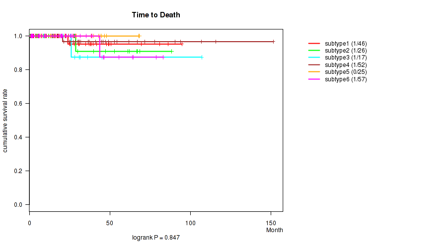
Testing the association between subtypes identified by 10 different clustering approaches and 14 clinical features across 367 patients, 37 significant findings detected with P value < 0.05 and Q value < 0.25.

3 subtypes identified in current cancer cohort by 'Copy Number Ratio CNMF subtypes'. These subtypes correlate to 'PATHOLOGY.T.STAGE', 'PATHOLOGY.N.STAGE', 'COMPLETENESS.OF.RESECTION', 'NUMBER.OF.LYMPH.NODES', 'GLEASON_SCORE_COMBINED', 'GLEASON_SCORE_PRIMARY', and 'GLEASON_SCORE'.
4 subtypes identified in current cancer cohort by 'METHLYATION CNMF'. These subtypes correlate to 'PATHOLOGY.T.STAGE', 'GLEASON_SCORE_COMBINED', 'GLEASON_SCORE_PRIMARY', and 'PSA_RESULT_PREOP'.
CNMF clustering analysis on RPPA data identified 3 subtypes that correlate to 'GLEASON_SCORE_COMBINED', 'GLEASON_SCORE_PRIMARY', and 'GLEASON_SCORE'.
Consensus hierarchical clustering analysis on RPPA data identified 3 subtypes that correlate to 'GLEASON_SCORE_COMBINED', 'GLEASON_SCORE_PRIMARY', and 'GLEASON_SCORE'.
CNMF clustering analysis on sequencing-based mRNA expression data identified 3 subtypes that do not correlate to any clinical features.
Consensus hierarchical clustering analysis on sequencing-based mRNA expression data identified 3 subtypes that do not correlate to any clinical features.
3 subtypes identified in current cancer cohort by 'MIRSEQ CNMF'. These subtypes correlate to 'PATHOLOGY.T.STAGE', 'NUMBER.OF.LYMPH.NODES', 'GLEASON_SCORE_COMBINED', 'GLEASON_SCORE_PRIMARY', and 'GLEASON_SCORE'.
5 subtypes identified in current cancer cohort by 'MIRSEQ CHIERARCHICAL'. These subtypes correlate to 'PATHOLOGY.T.STAGE', 'PATHOLOGY.N.STAGE', 'NUMBER.OF.LYMPH.NODES', 'GLEASON_SCORE_COMBINED', 'GLEASON_SCORE_PRIMARY', and 'GLEASON_SCORE'.
4 subtypes identified in current cancer cohort by 'MIRseq Mature CNMF subtypes'. These subtypes correlate to 'GLEASON_SCORE_COMBINED', 'GLEASON_SCORE_PRIMARY', and 'GLEASON_SCORE'.
6 subtypes identified in current cancer cohort by 'MIRseq Mature cHierClus subtypes'. These subtypes correlate to 'PATHOLOGY.T.STAGE', 'PATHOLOGY.N.STAGE', 'NUMBER.OF.LYMPH.NODES', 'GLEASON_SCORE_COMBINED', 'GLEASON_SCORE_PRIMARY', and 'GLEASON_SCORE'.

Results

Overview of the results

Table 1. Get Full Table Overview of the association between subtypes identified by 10 different clustering approaches and 14 clinical features. Shown in the table are P values (Q values). Thresholded by P value < 0.05 and Q value < 0.25, 37 significant findings detected.


Clinical Features	Statistical Tests	Copy Number Ratio CNMF subtypes	METHLYATION CNMF	RPPA CNMF subtypes	RPPA cHierClus subtypes	RNAseq CNMF subtypes	RNAseq cHierClus subtypes	MIRSEQ CNMF	MIRSEQ CHIERARCHICAL	MIRseq Mature CNMF subtypes	MIRseq Mature cHierClus subtypes
Time to Death	logrank test	0.95 (1.00)	0.391 (1.00)	100 (1.00)	100 (1.00)	0.441 (1.00)	0.439 (1.00)	0.208 (1.00)	0.913 (1.00)	0.753 (1.00)	0.847 (1.00)
AGE	Kruskal-Wallis (anova)	0.0127 (1.00)	0.00487 (0.477)	0.075 (1.00)	0.0144 (1.00)	0.486 (1.00)	0.226 (1.00)	0.268 (1.00)	0.333 (1.00)	0.235 (1.00)	0.363 (1.00)
PATHOLOGY T STAGE	Fisher's exact test	1e-05 (0.00131)	0.00014 (0.0169)	0.00501 (0.481)	0.0163 (1.00)	0.00314 (0.323)	0.0201 (1.00)	0.00048 (0.0552)	3e-05 (0.00375)	0.0465 (1.00)	0.00209 (0.222)
PATHOLOGY N STAGE	Fisher's exact test	0.00145 (0.155)	0.241 (1.00)	0.0544 (1.00)	0.0159 (1.00)	0.127 (1.00)	0.0377 (1.00)	0.00324 (0.33)	0.00091 (0.101)	0.392 (1.00)	0.00051 (0.0581)
HISTOLOGICAL TYPE	Fisher's exact test	0.586 (1.00)	0.509 (1.00)	1 (1.00)	0.337 (1.00)	0.683 (1.00)	0.94 (1.00)	0.0696 (1.00)	0.49 (1.00)	0.0582 (1.00)	0.148 (1.00)
COMPLETENESS OF RESECTION	Fisher's exact test	0.00067 (0.0757)	0.21 (1.00)	0.0246 (1.00)	0.00491 (0.477)	0.446 (1.00)	0.528 (1.00)	0.288 (1.00)	0.0486 (1.00)	0.0392 (1.00)	0.0355 (1.00)
NUMBER OF LYMPH NODES	Kruskal-Wallis (anova)	0.000349 (0.0408)	0.233 (1.00)	0.0381 (1.00)	0.0119 (1.00)	0.104 (1.00)	0.0268 (1.00)	0.00216 (0.227)	0.000816 (0.0914)	0.399 (1.00)	9.93e-05 (0.0121)
GLEASON SCORE COMBINED	Kruskal-Wallis (anova)	3.93e-13 (5.43e-11)	0.00227 (0.236)	6.61e-05 (0.00819)	2.96e-05 (0.00373)	0.0476 (1.00)	0.0215 (1.00)	2.91e-06 (0.000395)	6.91e-08 (9.46e-06)	0.0012 (0.129)	0.000367 (0.0426)
GLEASON SCORE PRIMARY	Kruskal-Wallis (anova)	3.13e-13 (4.35e-11)	0.00028 (0.0331)	1.13e-05 (0.00147)	8.3e-06 (0.0011)	0.00645 (0.6)	0.00463 (0.459)	6.44e-06 (0.000856)	2.31e-05 (0.00296)	0.00105 (0.114)	0.000278 (0.0331)
GLEASON SCORE SECONDARY	Kruskal-Wallis (anova)	0.00563 (0.529)	0.714 (1.00)	0.381 (1.00)	0.133 (1.00)	0.162 (1.00)	0.262 (1.00)	0.0237 (1.00)	0.0112 (0.984)	0.0799 (1.00)	0.121 (1.00)
GLEASON SCORE	Kruskal-Wallis (anova)	2.77e-16 (3.88e-14)	0.00325 (0.33)	2.81e-05 (0.00357)	4.5e-06 (0.000603)	0.00798 (0.718)	0.00552 (0.525)	1.31e-05 (0.00169)	3.13e-06 (0.000422)	0.000917 (0.101)	0.000186 (0.0223)
PSA RESULT PREOP	Kruskal-Wallis (anova)	0.00781 (0.714)	7.45e-05 (0.00917)	0.0455 (1.00)	0.0308 (1.00)	0.00327 (0.33)	0.00776 (0.714)	0.0607 (1.00)	0.321 (1.00)	0.432 (1.00)	0.0701 (1.00)
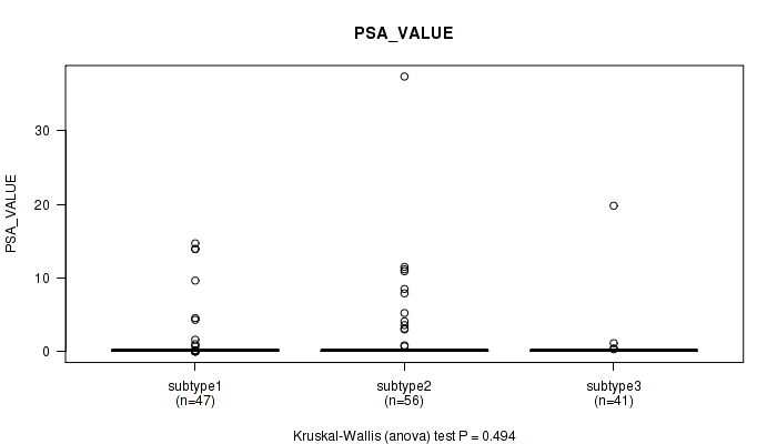
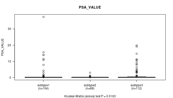
PSA VALUE	Kruskal-Wallis (anova)	0.47 (1.00)	0.51 (1.00)	0.193 (1.00)	0.494 (1.00)	0.114 (1.00)	0.31 (1.00)	0.0163 (1.00)	0.379 (1.00)	0.252 (1.00)	0.379 (1.00)
RACE	Fisher's exact test	0.565 (1.00)	0.361 (1.00)	0.0266 (1.00)	0.00843 (0.75)	0.0702 (1.00)	0.0656 (1.00)	0.218 (1.00)	0.706 (1.00)	0.806 (1.00)	0.803 (1.00)

Clustering Approach #1: 'Copy Number Ratio CNMF subtypes'

Table S1. Description of clustering approach #1: 'Copy Number Ratio CNMF subtypes'

Cluster Labels	1	2	3
Number of samples	207	88	68

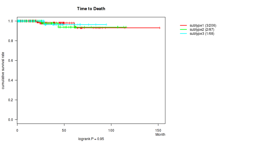
'Copy Number Ratio CNMF subtypes' versus 'Time to Death'

P value = 0.95 (logrank test), Q value = 1

Table S2. Clustering Approach #1: 'Copy Number Ratio CNMF subtypes' versus Clinical Feature #1: 'Time to Death'

	nPatients	nDeath	Duration Range (Median), Month
ALL	361	6	0.3 - 151.4 (23.9)
subtype1	206	3	0.7 - 151.4 (21.9)
subtype2	87	2	0.8 - 115.9 (26.5)
subtype3	68	1	0.3 - 94.7 (25.3)

Figure S1. Get High-res Image Clustering Approach #1: 'Copy Number Ratio CNMF subtypes' versus Clinical Feature #1: 'Time to Death'

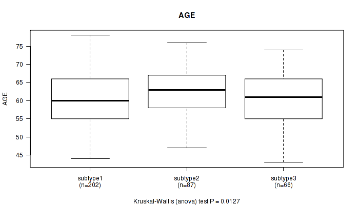
'Copy Number Ratio CNMF subtypes' versus 'AGE'

P value = 0.0127 (Kruskal-Wallis (anova)), Q value = 1

Table S3. Clustering Approach #1: 'Copy Number Ratio CNMF subtypes' versus Clinical Feature #2: 'AGE'

	nPatients	Mean (Std.Dev)
ALL	355	60.8 (7.0)
subtype1	202	60.2 (7.0)
subtype2	87	62.7 (5.9)
subtype3	66	60.2 (7.7)

Figure S2. Get High-res Image Clustering Approach #1: 'Copy Number Ratio CNMF subtypes' versus Clinical Feature #2: 'AGE'

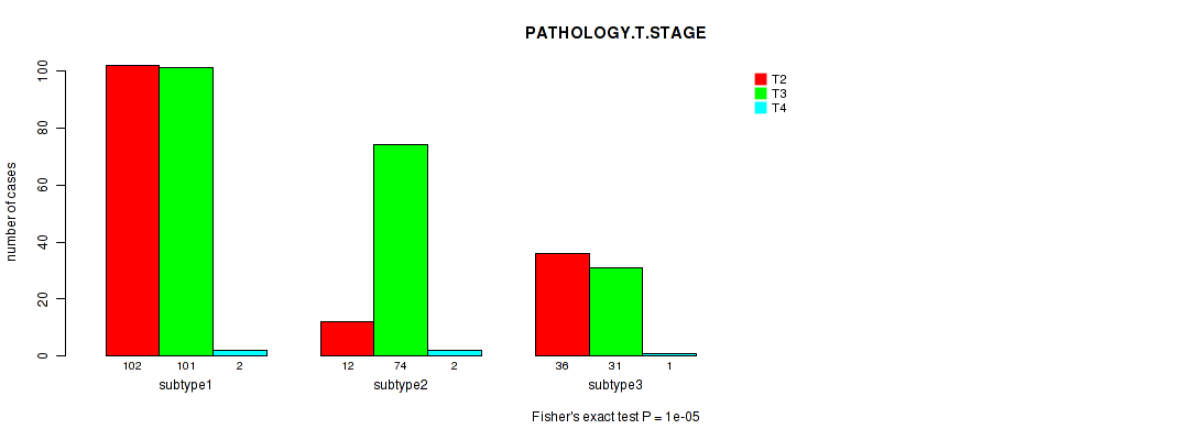
'Copy Number Ratio CNMF subtypes' versus 'PATHOLOGY.T.STAGE'

P value = 1e-05 (Fisher's exact test), Q value = 0.0013

Table S4. Clustering Approach #1: 'Copy Number Ratio CNMF subtypes' versus Clinical Feature #3: 'PATHOLOGY.T.STAGE'

nPatients	T2	T3	T4
ALL	150	206	5
subtype1	102	101	2
subtype2	12	74	2
subtype3	36	31	1

Figure S3. Get High-res Image Clustering Approach #1: 'Copy Number Ratio CNMF subtypes' versus Clinical Feature #3: 'PATHOLOGY.T.STAGE'

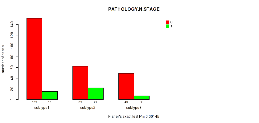
'Copy Number Ratio CNMF subtypes' versus 'PATHOLOGY.N.STAGE'

P value = 0.00145 (Fisher's exact test), Q value = 0.16

Table S5. Clustering Approach #1: 'Copy Number Ratio CNMF subtypes' versus Clinical Feature #4: 'PATHOLOGY.N.STAGE'

nPatients	0	1
ALL	263	44
subtype1	152	15
subtype2	62	22
subtype3	49	7

Figure S4. Get High-res Image Clustering Approach #1: 'Copy Number Ratio CNMF subtypes' versus Clinical Feature #4: 'PATHOLOGY.N.STAGE'

'Copy Number Ratio CNMF subtypes' versus 'HISTOLOGICAL.TYPE'

P value = 0.586 (Fisher's exact test), Q value = 1

Table S6. Clustering Approach #1: 'Copy Number Ratio CNMF subtypes' versus Clinical Feature #5: 'HISTOLOGICAL.TYPE'

nPatients	PROSTATE ADENOCARCINOMA OTHER SUBTYPE	PROSTATE ADENOCARCINOMA ACINAR TYPE
ALL	13	350
subtype1	8	199
subtype2	4	84
subtype3	1	67

Figure S5. Get High-res Image Clustering Approach #1: 'Copy Number Ratio CNMF subtypes' versus Clinical Feature #5: 'HISTOLOGICAL.TYPE'

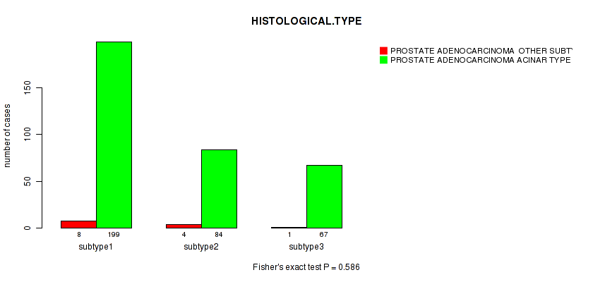
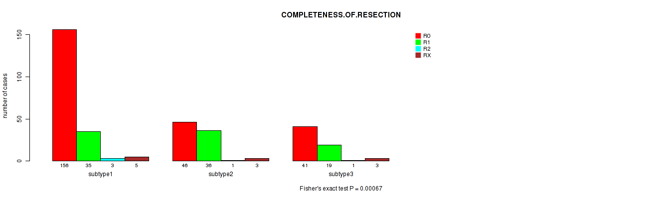
'Copy Number Ratio CNMF subtypes' versus 'COMPLETENESS.OF.RESECTION'

P value = 0.00067 (Fisher's exact test), Q value = 0.076

Table S7. Clustering Approach #1: 'Copy Number Ratio CNMF subtypes' versus Clinical Feature #6: 'COMPLETENESS.OF.RESECTION'

nPatients	R0	R1	R2	RX
ALL	243	90	5	11
subtype1	156	35	3	5
subtype2	46	36	1	3
subtype3	41	19	1	3

Figure S6. Get High-res Image Clustering Approach #1: 'Copy Number Ratio CNMF subtypes' versus Clinical Feature #6: 'COMPLETENESS.OF.RESECTION'

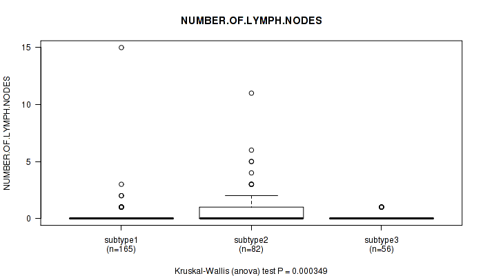
'Copy Number Ratio CNMF subtypes' versus 'NUMBER.OF.LYMPH.NODES'

P value = 0.000349 (Kruskal-Wallis (anova)), Q value = 0.041

Table S8. Clustering Approach #1: 'Copy Number Ratio CNMF subtypes' versus Clinical Feature #7: 'NUMBER.OF.LYMPH.NODES'

	nPatients	Mean (Std.Dev)
ALL	303	0.3 (1.3)
subtype1	165	0.2 (1.2)
subtype2	82	0.7 (1.7)
subtype3	56	0.1 (0.3)

Figure S7. Get High-res Image Clustering Approach #1: 'Copy Number Ratio CNMF subtypes' versus Clinical Feature #7: 'NUMBER.OF.LYMPH.NODES'

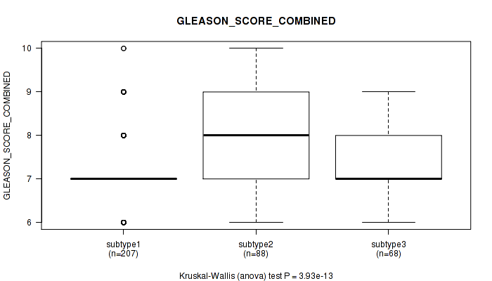
'Copy Number Ratio CNMF subtypes' versus 'GLEASON_SCORE_COMBINED'

P value = 3.93e-13 (Kruskal-Wallis (anova)), Q value = 5.4e-11

Table S9. Clustering Approach #1: 'Copy Number Ratio CNMF subtypes' versus Clinical Feature #8: 'GLEASON_SCORE_COMBINED'

	nPatients	Mean (Std.Dev)
ALL	363	7.4 (0.9)
subtype1	207	7.2 (0.8)
subtype2	88	8.1 (0.9)
subtype3	68	7.3 (0.8)

Figure S8. Get High-res Image Clustering Approach #1: 'Copy Number Ratio CNMF subtypes' versus Clinical Feature #8: 'GLEASON_SCORE_COMBINED'

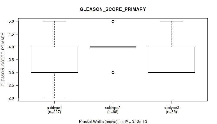
'Copy Number Ratio CNMF subtypes' versus 'GLEASON_SCORE_PRIMARY'

P value = 3.13e-13 (Kruskal-Wallis (anova)), Q value = 4.4e-11

Table S10. Clustering Approach #1: 'Copy Number Ratio CNMF subtypes' versus Clinical Feature #9: 'GLEASON_SCORE_PRIMARY'

	nPatients	Mean (Std.Dev)
ALL	363	3.6 (0.6)
subtype1	207	3.5 (0.6)
subtype2	88	4.0 (0.6)
subtype3	68	3.5 (0.6)

Figure S9. Get High-res Image Clustering Approach #1: 'Copy Number Ratio CNMF subtypes' versus Clinical Feature #9: 'GLEASON_SCORE_PRIMARY'

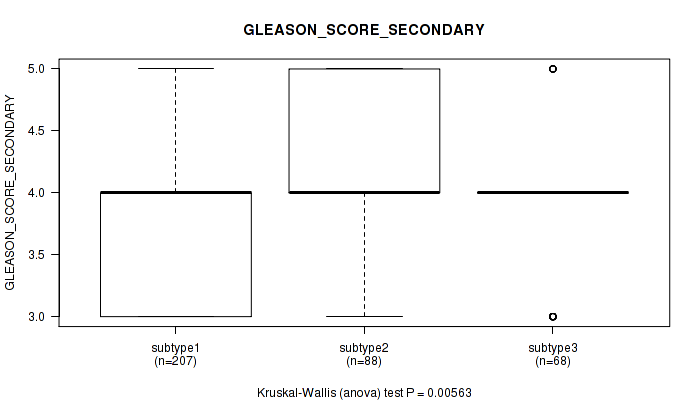
'Copy Number Ratio CNMF subtypes' versus 'GLEASON_SCORE_SECONDARY'

P value = 0.00563 (Kruskal-Wallis (anova)), Q value = 0.53

Table S11. Clustering Approach #1: 'Copy Number Ratio CNMF subtypes' versus Clinical Feature #10: 'GLEASON_SCORE_SECONDARY'

	nPatients	Mean (Std.Dev)
ALL	363	3.9 (0.6)
subtype1	207	3.8 (0.6)
subtype2	88	4.0 (0.7)
subtype3	68	3.9 (0.6)

Figure S10. Get High-res Image Clustering Approach #1: 'Copy Number Ratio CNMF subtypes' versus Clinical Feature #10: 'GLEASON_SCORE_SECONDARY'

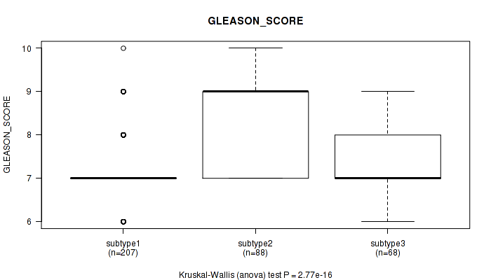
'Copy Number Ratio CNMF subtypes' versus 'GLEASON_SCORE'

P value = 2.77e-16 (Kruskal-Wallis (anova)), Q value = 3.9e-14

Table S12. Clustering Approach #1: 'Copy Number Ratio CNMF subtypes' versus Clinical Feature #11: 'GLEASON_SCORE'

	nPatients	Mean (Std.Dev)
ALL	363	7.5 (1.0)
subtype1	207	7.2 (0.8)
subtype2	88	8.3 (0.9)
subtype3	68	7.4 (0.8)

Figure S11. Get High-res Image Clustering Approach #1: 'Copy Number Ratio CNMF subtypes' versus Clinical Feature #11: 'GLEASON_SCORE'

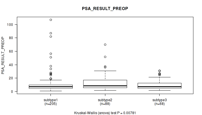
'Copy Number Ratio CNMF subtypes' versus 'PSA_RESULT_PREOP'

P value = 0.00781 (Kruskal-Wallis (anova)), Q value = 0.71

Table S13. Clustering Approach #1: 'Copy Number Ratio CNMF subtypes' versus Clinical Feature #12: 'PSA_RESULT_PREOP'

	nPatients	Mean (Std.Dev)
ALL	361	10.5 (11.3)
subtype1	205	9.7 (12.3)
subtype2	88	12.8 (11.3)
subtype3	68	9.8 (7.1)

Figure S12. Get High-res Image Clustering Approach #1: 'Copy Number Ratio CNMF subtypes' versus Clinical Feature #12: 'PSA_RESULT_PREOP'

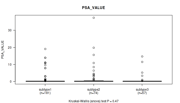
'Copy Number Ratio CNMF subtypes' versus 'PSA_VALUE'

P value = 0.47 (Kruskal-Wallis (anova)), Q value = 1

Table S14. Clustering Approach #1: 'Copy Number Ratio CNMF subtypes' versus Clinical Feature #13: 'PSA_VALUE'

	nPatients	Mean (Std.Dev)
ALL	312	1.0 (3.5)
subtype1	181	0.8 (2.6)
subtype2	74	1.7 (5.4)
subtype3	57	0.7 (2.5)

Figure S13. Get High-res Image Clustering Approach #1: 'Copy Number Ratio CNMF subtypes' versus Clinical Feature #13: 'PSA_VALUE'

'Copy Number Ratio CNMF subtypes' versus 'RACE'

P value = 0.565 (Fisher's exact test), Q value = 1

Table S15. Clustering Approach #1: 'Copy Number Ratio CNMF subtypes' versus Clinical Feature #14: 'RACE'

nPatients	ASIAN	BLACK OR AFRICAN AMERICAN	WHITE
ALL	2	7	146
subtype1	2	3	90
subtype2	0	1	29
subtype3	0	3	27

Figure S14. Get High-res Image Clustering Approach #1: 'Copy Number Ratio CNMF subtypes' versus Clinical Feature #14: 'RACE'

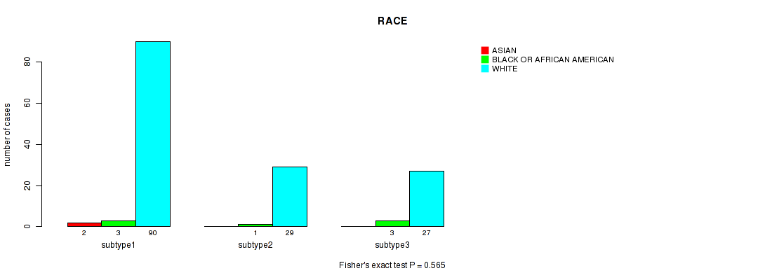
Clustering Approach #2: 'METHLYATION CNMF'

Table S16. Description of clustering approach #2: 'METHLYATION CNMF'

Cluster Labels	1	2	3	4
Number of samples	109	102	104	30

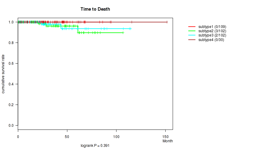
'METHLYATION CNMF' versus 'Time to Death'

P value = 0.391 (logrank test), Q value = 1

Table S17. Clustering Approach #2: 'METHLYATION CNMF' versus Clinical Feature #1: 'Time to Death'

	nPatients	nDeath	Duration Range (Median), Month
ALL	343	5	0.3 - 151.4 (23.0)
subtype1	109	0	1.1 - 94.7 (20.5)
subtype2	102	3	0.3 - 106.8 (27.0)
subtype3	102	2	1.0 - 114.6 (22.2)
subtype4	30	0	1.6 - 151.4 (25.6)

Figure S15. Get High-res Image Clustering Approach #2: 'METHLYATION CNMF' versus Clinical Feature #1: 'Time to Death'

'METHLYATION CNMF' versus 'AGE'

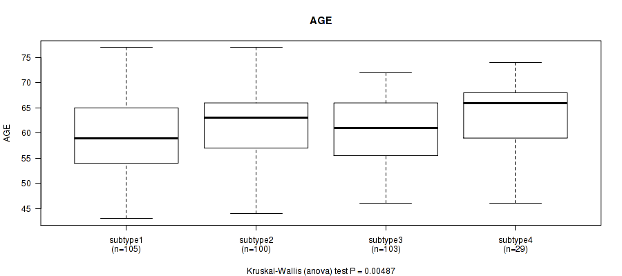
P value = 0.00487 (Kruskal-Wallis (anova)), Q value = 0.48

Table S18. Clustering Approach #2: 'METHLYATION CNMF' versus Clinical Feature #2: 'AGE'

	nPatients	Mean (Std.Dev)
ALL	337	60.7 (6.9)
subtype1	105	59.2 (6.8)
subtype2	100	61.9 (6.9)
subtype3	103	60.5 (6.8)
subtype4	29	63.0 (6.7)

Figure S16. Get High-res Image Clustering Approach #2: 'METHLYATION CNMF' versus Clinical Feature #2: 'AGE'

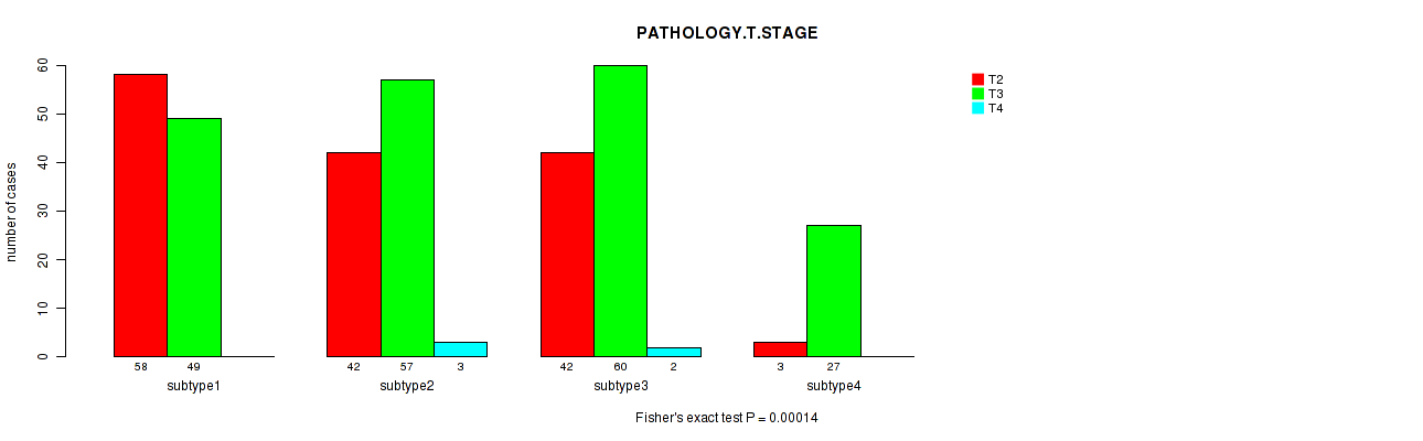
'METHLYATION CNMF' versus 'PATHOLOGY.T.STAGE'

P value = 0.00014 (Fisher's exact test), Q value = 0.017

Table S19. Clustering Approach #2: 'METHLYATION CNMF' versus Clinical Feature #3: 'PATHOLOGY.T.STAGE'

nPatients	T2	T3	T4
ALL	145	193	5
subtype1	58	49	0
subtype2	42	57	3
subtype3	42	60	2
subtype4	3	27	0

Figure S17. Get High-res Image Clustering Approach #2: 'METHLYATION CNMF' versus Clinical Feature #3: 'PATHOLOGY.T.STAGE'

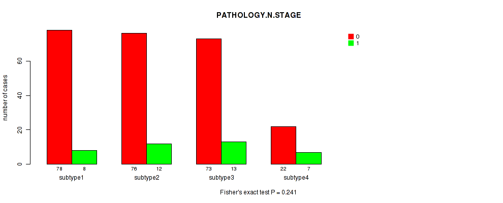
'METHLYATION CNMF' versus 'PATHOLOGY.N.STAGE'

P value = 0.241 (Fisher's exact test), Q value = 1

Table S20. Clustering Approach #2: 'METHLYATION CNMF' versus Clinical Feature #4: 'PATHOLOGY.N.STAGE'

nPatients	0	1
ALL	249	40
subtype1	78	8
subtype2	76	12
subtype3	73	13
subtype4	22	7

Figure S18. Get High-res Image Clustering Approach #2: 'METHLYATION CNMF' versus Clinical Feature #4: 'PATHOLOGY.N.STAGE'

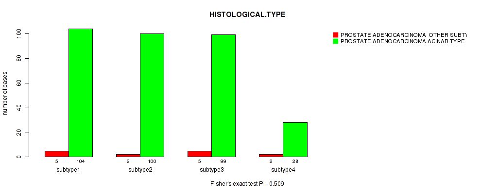
'METHLYATION CNMF' versus 'HISTOLOGICAL.TYPE'

P value = 0.509 (Fisher's exact test), Q value = 1

Table S21. Clustering Approach #2: 'METHLYATION CNMF' versus Clinical Feature #5: 'HISTOLOGICAL.TYPE'

nPatients	PROSTATE ADENOCARCINOMA OTHER SUBTYPE	PROSTATE ADENOCARCINOMA ACINAR TYPE
ALL	14	331
subtype1	5	104
subtype2	2	100
subtype3	5	99
subtype4	2	28

Figure S19. Get High-res Image Clustering Approach #2: 'METHLYATION CNMF' versus Clinical Feature #5: 'HISTOLOGICAL.TYPE'

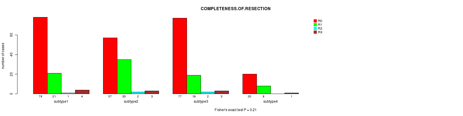
'METHLYATION CNMF' versus 'COMPLETENESS.OF.RESECTION'

P value = 0.21 (Fisher's exact test), Q value = 1

Table S22. Clustering Approach #2: 'METHLYATION CNMF' versus Clinical Feature #6: 'COMPLETENESS.OF.RESECTION'

nPatients	R0	R1	R2	RX
ALL	232	83	5	11
subtype1	78	21	1	4
subtype2	57	35	2	3
subtype3	77	19	2	3
subtype4	20	8	0	1

Figure S20. Get High-res Image Clustering Approach #2: 'METHLYATION CNMF' versus Clinical Feature #6: 'COMPLETENESS.OF.RESECTION'

'METHLYATION CNMF' versus 'NUMBER.OF.LYMPH.NODES'

P value = 0.233 (Kruskal-Wallis (anova)), Q value = 1

Table S23. Clustering Approach #2: 'METHLYATION CNMF' versus Clinical Feature #7: 'NUMBER.OF.LYMPH.NODES'

	nPatients	Mean (Std.Dev)
ALL	285	0.3 (1.1)
subtype1	84	0.1 (0.5)
subtype2	86	0.2 (0.5)
subtype3	86	0.5 (1.9)
subtype4	29	0.4 (0.8)

Figure S21. Get High-res Image Clustering Approach #2: 'METHLYATION CNMF' versus Clinical Feature #7: 'NUMBER.OF.LYMPH.NODES'

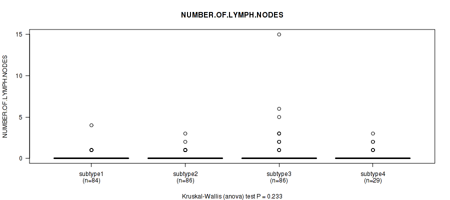
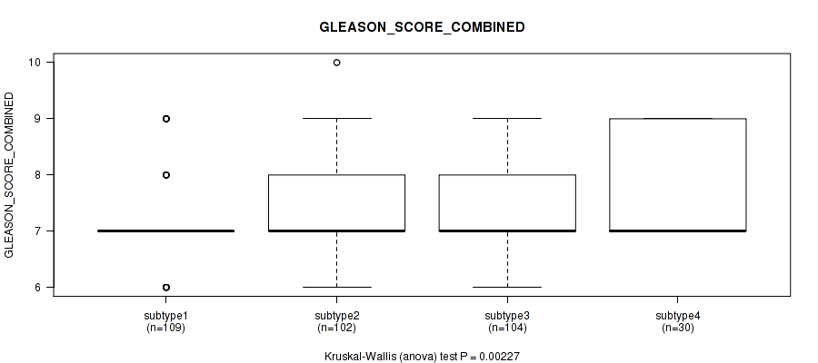
'METHLYATION CNMF' versus 'GLEASON_SCORE_COMBINED'

P value = 0.00227 (Kruskal-Wallis (anova)), Q value = 0.24

Table S24. Clustering Approach #2: 'METHLYATION CNMF' versus Clinical Feature #8: 'GLEASON_SCORE_COMBINED'

	nPatients	Mean (Std.Dev)
ALL	345	7.4 (0.9)
subtype1	109	7.2 (0.8)
subtype2	102	7.6 (1.0)
subtype3	104	7.4 (0.9)
subtype4	30	7.7 (0.9)

Figure S22. Get High-res Image Clustering Approach #2: 'METHLYATION CNMF' versus Clinical Feature #8: 'GLEASON_SCORE_COMBINED'

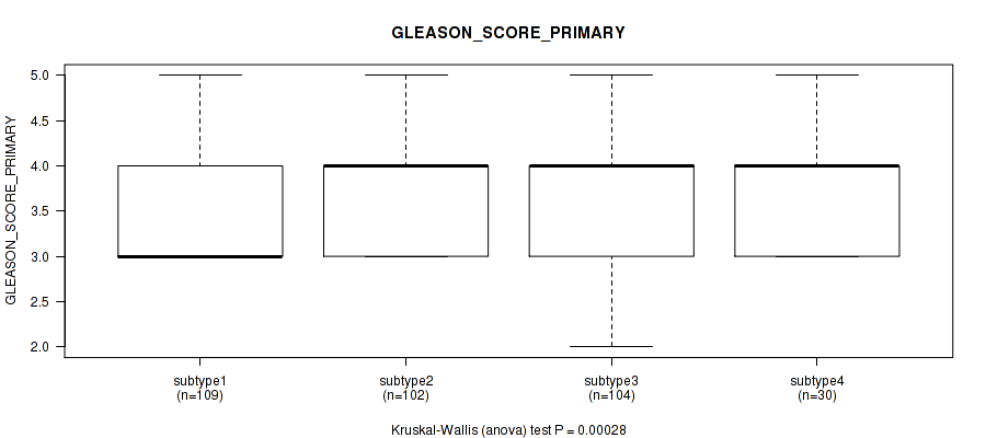
'METHLYATION CNMF' versus 'GLEASON_SCORE_PRIMARY'

P value = 0.00028 (Kruskal-Wallis (anova)), Q value = 0.033

Table S25. Clustering Approach #2: 'METHLYATION CNMF' versus Clinical Feature #9: 'GLEASON_SCORE_PRIMARY'

	nPatients	Mean (Std.Dev)
ALL	345	3.6 (0.6)
subtype1	109	3.4 (0.5)
subtype2	102	3.7 (0.6)
subtype3	104	3.5 (0.6)
subtype4	30	3.8 (0.5)

Figure S23. Get High-res Image Clustering Approach #2: 'METHLYATION CNMF' versus Clinical Feature #9: 'GLEASON_SCORE_PRIMARY'

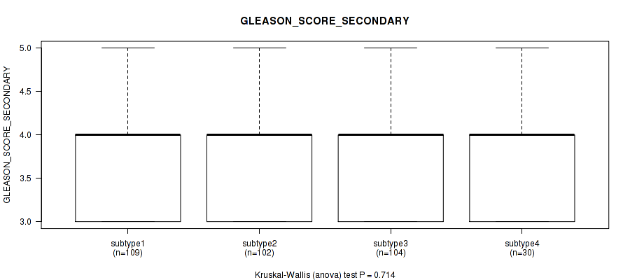
'METHLYATION CNMF' versus 'GLEASON_SCORE_SECONDARY'

P value = 0.714 (Kruskal-Wallis (anova)), Q value = 1

Table S26. Clustering Approach #2: 'METHLYATION CNMF' versus Clinical Feature #10: 'GLEASON_SCORE_SECONDARY'

	nPatients	Mean (Std.Dev)
ALL	345	3.9 (0.7)
subtype1	109	3.8 (0.6)
subtype2	102	3.9 (0.7)
subtype3	104	3.8 (0.6)
subtype4	30	3.9 (0.7)

Figure S24. Get High-res Image Clustering Approach #2: 'METHLYATION CNMF' versus Clinical Feature #10: 'GLEASON_SCORE_SECONDARY'

'METHLYATION CNMF' versus 'GLEASON_SCORE'

P value = 0.00325 (Kruskal-Wallis (anova)), Q value = 0.33

Table S27. Clustering Approach #2: 'METHLYATION CNMF' versus Clinical Feature #11: 'GLEASON_SCORE'

	nPatients	Mean (Std.Dev)
ALL	345	7.5 (0.9)
subtype1	109	7.2 (0.8)
subtype2	102	7.7 (1.0)
subtype3	104	7.5 (0.9)
subtype4	30	7.8 (0.9)

Figure S25. Get High-res Image Clustering Approach #2: 'METHLYATION CNMF' versus Clinical Feature #11: 'GLEASON_SCORE'

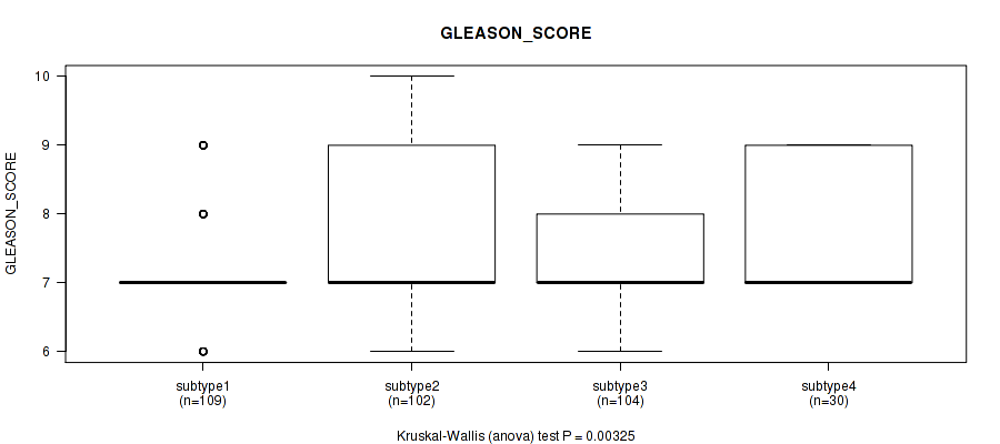
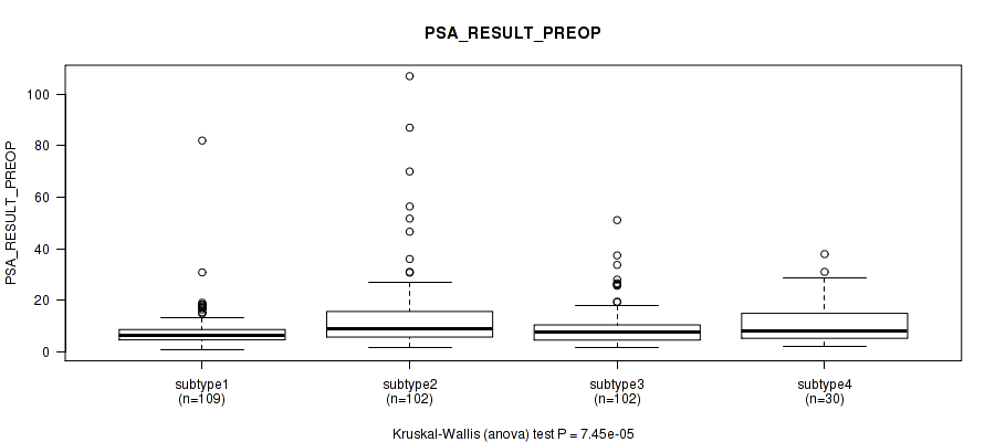
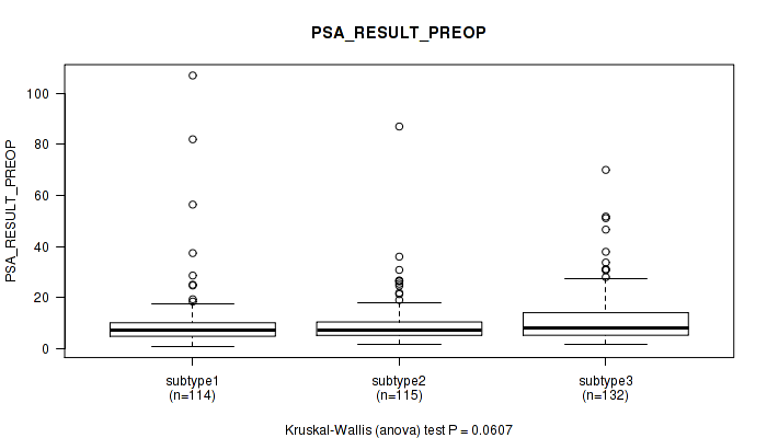
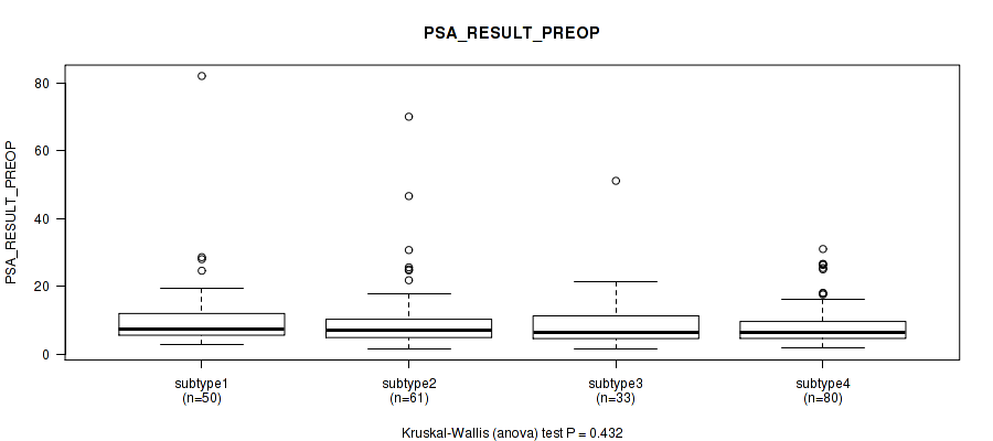
'METHLYATION CNMF' versus 'PSA_RESULT_PREOP'

P value = 7.45e-05 (Kruskal-Wallis (anova)), Q value = 0.0092

Table S28. Clustering Approach #2: 'METHLYATION CNMF' versus Clinical Feature #12: 'PSA_RESULT_PREOP'

	nPatients	Mean (Std.Dev)
ALL	343	10.8 (11.7)
subtype1	109	8.1 (8.4)
subtype2	102	14.7 (16.5)
subtype3	102	9.4 (7.9)
subtype4	30	11.6 (9.4)

Figure S26. Get High-res Image Clustering Approach #2: 'METHLYATION CNMF' versus Clinical Feature #12: 'PSA_RESULT_PREOP'

'METHLYATION CNMF' versus 'PSA_VALUE'

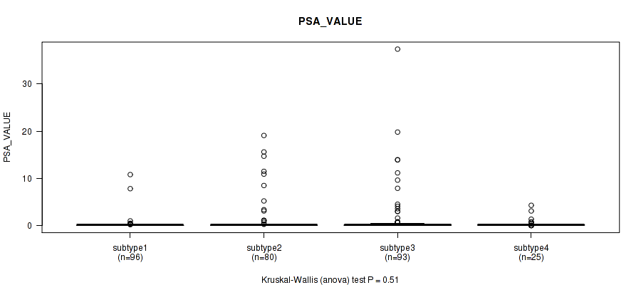
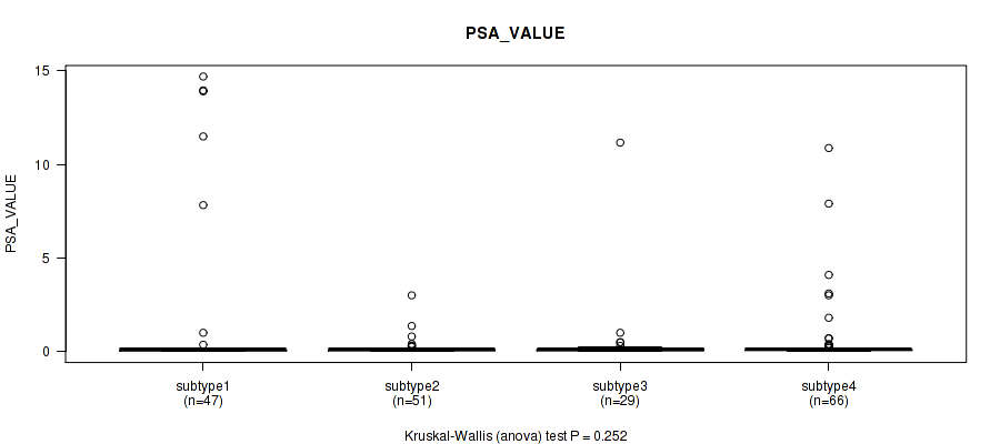
P value = 0.51 (Kruskal-Wallis (anova)), Q value = 1

Table S29. Clustering Approach #2: 'METHLYATION CNMF' versus Clinical Feature #13: 'PSA_VALUE'

	nPatients	Mean (Std.Dev)
ALL	294	1.0 (3.5)
subtype1	96	0.3 (1.3)
subtype2	80	1.3 (3.7)
subtype3	93	1.5 (5.0)
subtype4	25	0.5 (1.0)

Figure S27. Get High-res Image Clustering Approach #2: 'METHLYATION CNMF' versus Clinical Feature #13: 'PSA_VALUE'

'METHLYATION CNMF' versus 'RACE'

P value = 0.361 (Fisher's exact test), Q value = 1

Table S30. Clustering Approach #2: 'METHLYATION CNMF' versus Clinical Feature #14: 'RACE'

nPatients	ASIAN	BLACK OR AFRICAN AMERICAN	WHITE
ALL	2	7	147
subtype1	1	2	47
subtype2	0	1	38
subtype3	0	3	51
subtype4	1	1	11

Figure S28. Get High-res Image Clustering Approach #2: 'METHLYATION CNMF' versus Clinical Feature #14: 'RACE'

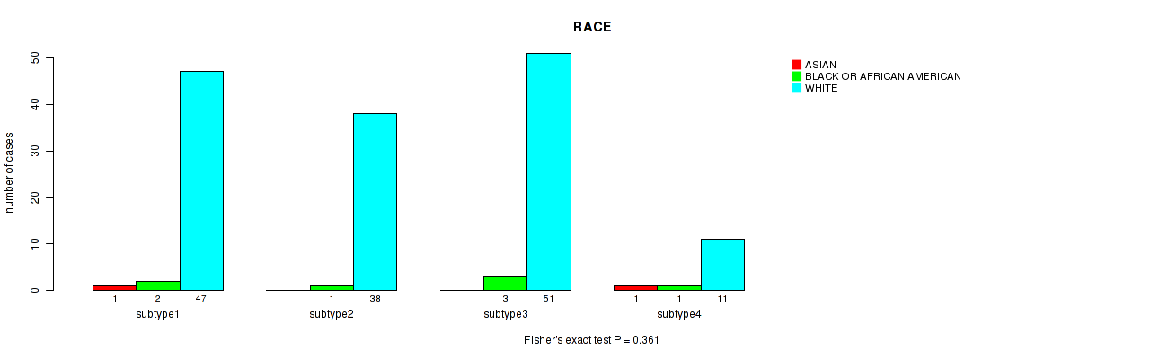
Clustering Approach #3: 'RPPA CNMF subtypes'

Table S31. Description of clustering approach #3: 'RPPA CNMF subtypes'

Cluster Labels	1	2	3
Number of samples	42	55	62

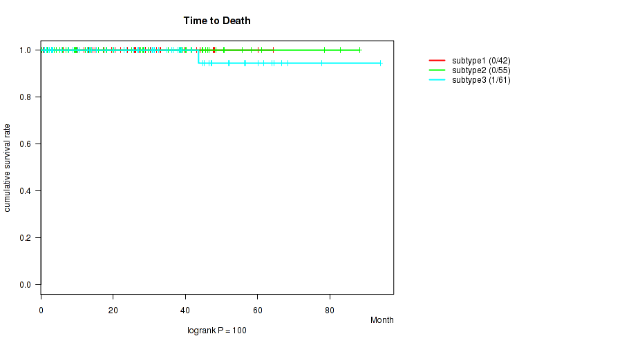
'RPPA CNMF subtypes' versus 'Time to Death'

P value = 100 (logrank test), Q value = 1

Table S32. Clustering Approach #3: 'RPPA CNMF subtypes' versus Clinical Feature #1: 'Time to Death'

	nPatients	nDeath	Duration Range (Median), Month
ALL	158	1	0.3 - 94.0 (27.0)
subtype1	42	0	0.7 - 64.5 (25.0)
subtype2	55	0	0.3 - 88.2 (27.0)
subtype3	61	1	0.8 - 94.0 (30.5)

Figure S29. Get High-res Image Clustering Approach #3: 'RPPA CNMF subtypes' versus Clinical Feature #1: 'Time to Death'

'RPPA CNMF subtypes' versus 'AGE'

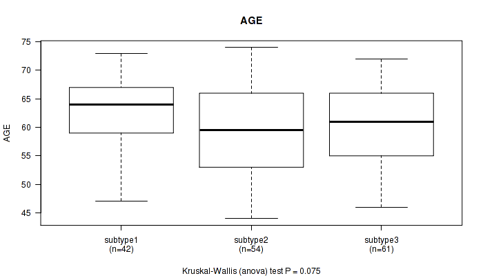
P value = 0.075 (Kruskal-Wallis (anova)), Q value = 1

Table S33. Clustering Approach #3: 'RPPA CNMF subtypes' versus Clinical Feature #2: 'AGE'

	nPatients	Mean (Std.Dev)
ALL	157	60.6 (7.1)
subtype1	42	62.7 (6.3)
subtype2	54	59.2 (7.8)
subtype3	61	60.3 (6.7)

Figure S30. Get High-res Image Clustering Approach #3: 'RPPA CNMF subtypes' versus Clinical Feature #2: 'AGE'

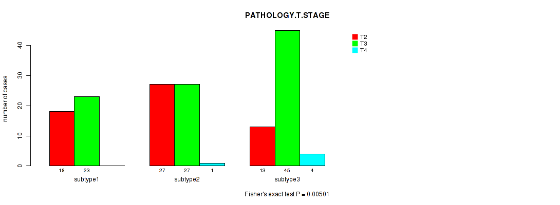
'RPPA CNMF subtypes' versus 'PATHOLOGY.T.STAGE'

P value = 0.00501 (Fisher's exact test), Q value = 0.48

Table S34. Clustering Approach #3: 'RPPA CNMF subtypes' versus Clinical Feature #3: 'PATHOLOGY.T.STAGE'

nPatients	T2	T3	T4
ALL	58	95	5
subtype1	18	23	0
subtype2	27	27	1
subtype3	13	45	4

Figure S31. Get High-res Image Clustering Approach #3: 'RPPA CNMF subtypes' versus Clinical Feature #3: 'PATHOLOGY.T.STAGE'

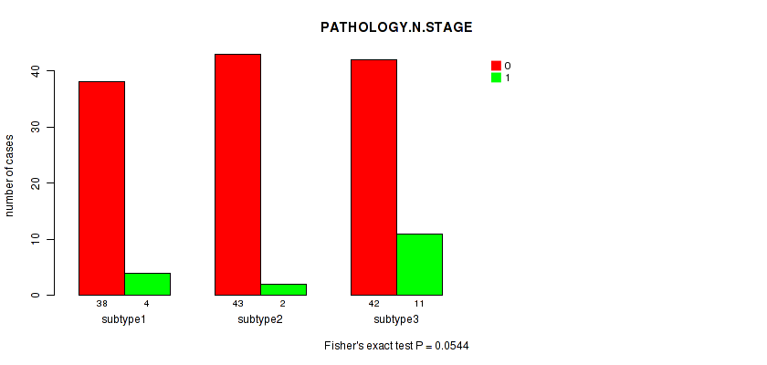
'RPPA CNMF subtypes' versus 'PATHOLOGY.N.STAGE'

P value = 0.0544 (Fisher's exact test), Q value = 1

Table S35. Clustering Approach #3: 'RPPA CNMF subtypes' versus Clinical Feature #4: 'PATHOLOGY.N.STAGE'

nPatients	0	1
ALL	123	17
subtype1	38	4
subtype2	43	2
subtype3	42	11

Figure S32. Get High-res Image Clustering Approach #3: 'RPPA CNMF subtypes' versus Clinical Feature #4: 'PATHOLOGY.N.STAGE'

'RPPA CNMF subtypes' versus 'HISTOLOGICAL.TYPE'

P value = 1 (Fisher's exact test), Q value = 1

Table S36. Clustering Approach #3: 'RPPA CNMF subtypes' versus Clinical Feature #5: 'HISTOLOGICAL.TYPE'

nPatients	PROSTATE ADENOCARCINOMA OTHER SUBTYPE	PROSTATE ADENOCARCINOMA ACINAR TYPE
ALL	2	157
subtype1	0	42
subtype2	1	54
subtype3	1	61

Figure S33. Get High-res Image Clustering Approach #3: 'RPPA CNMF subtypes' versus Clinical Feature #5: 'HISTOLOGICAL.TYPE'

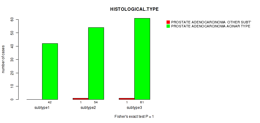
'RPPA CNMF subtypes' versus 'COMPLETENESS.OF.RESECTION'

P value = 0.0246 (Fisher's exact test), Q value = 1

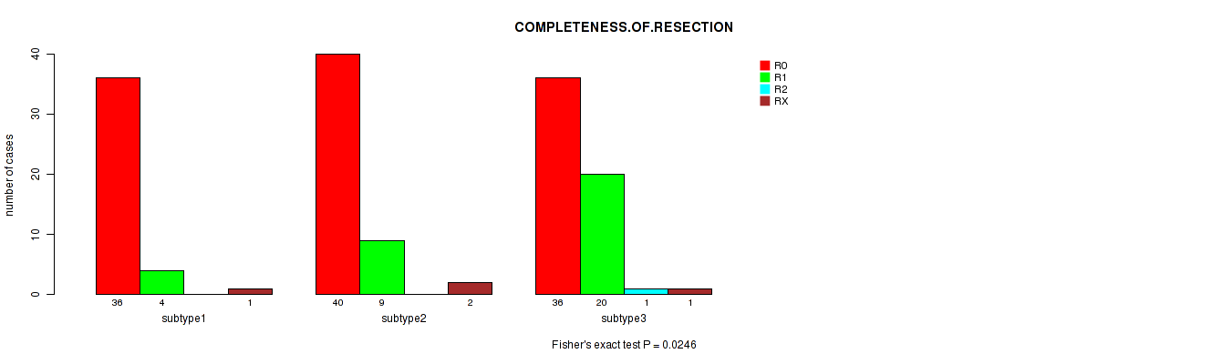
Table S37. Clustering Approach #3: 'RPPA CNMF subtypes' versus Clinical Feature #6: 'COMPLETENESS.OF.RESECTION'

nPatients	R0	R1	R2	RX
ALL	112	33	1	4
subtype1	36	4	0	1
subtype2	40	9	0	2
subtype3	36	20	1	1

Figure S34. Get High-res Image Clustering Approach #3: 'RPPA CNMF subtypes' versus Clinical Feature #6: 'COMPLETENESS.OF.RESECTION'

'RPPA CNMF subtypes' versus 'NUMBER.OF.LYMPH.NODES'

P value = 0.0381 (Kruskal-Wallis (anova)), Q value = 1

Table S38. Clustering Approach #3: 'RPPA CNMF subtypes' versus Clinical Feature #7: 'NUMBER.OF.LYMPH.NODES'

	nPatients	Mean (Std.Dev)
ALL	140	0.2 (0.7)
subtype1	42	0.1 (0.5)
subtype2	45	0.1 (0.3)
subtype3	53	0.4 (1.1)

Figure S35. Get High-res Image Clustering Approach #3: 'RPPA CNMF subtypes' versus Clinical Feature #7: 'NUMBER.OF.LYMPH.NODES'

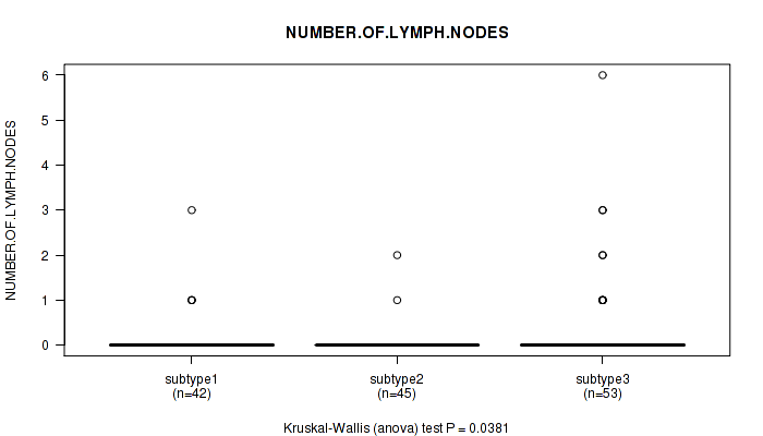
'RPPA CNMF subtypes' versus 'GLEASON_SCORE_COMBINED'

P value = 6.61e-05 (Kruskal-Wallis (anova)), Q value = 0.0082

Table S39. Clustering Approach #3: 'RPPA CNMF subtypes' versus Clinical Feature #8: 'GLEASON_SCORE_COMBINED'

	nPatients	Mean (Std.Dev)
ALL	159	7.4 (0.9)
subtype1	42	7.1 (0.5)
subtype2	55	7.3 (0.8)
subtype3	62	7.8 (1.0)

Figure S36. Get High-res Image Clustering Approach #3: 'RPPA CNMF subtypes' versus Clinical Feature #8: 'GLEASON_SCORE_COMBINED'

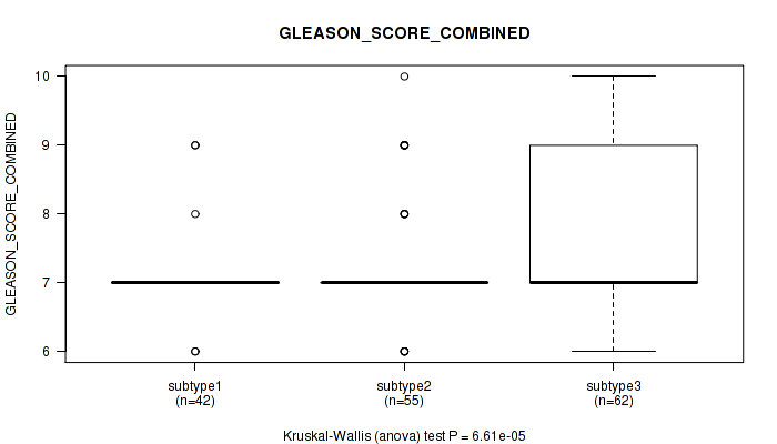
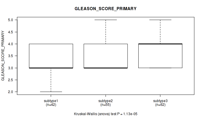
'RPPA CNMF subtypes' versus 'GLEASON_SCORE_PRIMARY'

P value = 1.13e-05 (Kruskal-Wallis (anova)), Q value = 0.0015

Table S40. Clustering Approach #3: 'RPPA CNMF subtypes' versus Clinical Feature #9: 'GLEASON_SCORE_PRIMARY'

	nPatients	Mean (Std.Dev)
ALL	159	3.5 (0.6)
subtype1	42	3.3 (0.5)
subtype2	55	3.4 (0.5)
subtype3	62	3.8 (0.6)

Figure S37. Get High-res Image Clustering Approach #3: 'RPPA CNMF subtypes' versus Clinical Feature #9: 'GLEASON_SCORE_PRIMARY'

'RPPA CNMF subtypes' versus 'GLEASON_SCORE_SECONDARY'

P value = 0.381 (Kruskal-Wallis (anova)), Q value = 1

Table S41. Clustering Approach #3: 'RPPA CNMF subtypes' versus Clinical Feature #10: 'GLEASON_SCORE_SECONDARY'

	nPatients	Mean (Std.Dev)
ALL	159	3.9 (0.7)
subtype1	42	3.7 (0.5)
subtype2	55	3.9 (0.7)
subtype3	62	4.0 (0.8)

Figure S38. Get High-res Image Clustering Approach #3: 'RPPA CNMF subtypes' versus Clinical Feature #10: 'GLEASON_SCORE_SECONDARY'

'RPPA CNMF subtypes' versus 'GLEASON_SCORE'

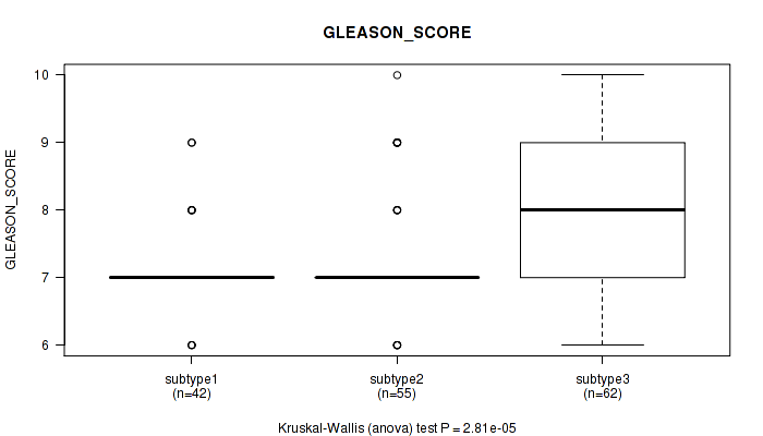
P value = 2.81e-05 (Kruskal-Wallis (anova)), Q value = 0.0036

Table S42. Clustering Approach #3: 'RPPA CNMF subtypes' versus Clinical Feature #11: 'GLEASON_SCORE'

	nPatients	Mean (Std.Dev)
ALL	159	7.5 (0.9)
subtype1	42	7.1 (0.6)
subtype2	55	7.3 (0.8)
subtype3	62	7.9 (1.0)

Figure S39. Get High-res Image Clustering Approach #3: 'RPPA CNMF subtypes' versus Clinical Feature #11: 'GLEASON_SCORE'

'RPPA CNMF subtypes' versus 'PSA_RESULT_PREOP'

P value = 0.0455 (Kruskal-Wallis (anova)), Q value = 1

Table S43. Clustering Approach #3: 'RPPA CNMF subtypes' versus Clinical Feature #12: 'PSA_RESULT_PREOP'

	nPatients	Mean (Std.Dev)
ALL	157	11.2 (11.2)
subtype1	41	8.3 (5.0)
subtype2	54	10.5 (13.4)
subtype3	62	13.9 (11.6)

Figure S40. Get High-res Image Clustering Approach #3: 'RPPA CNMF subtypes' versus Clinical Feature #12: 'PSA_RESULT_PREOP'

'RPPA CNMF subtypes' versus 'PSA_VALUE'

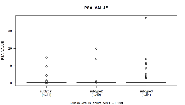
P value = 0.193 (Kruskal-Wallis (anova)), Q value = 1

Table S44. Clustering Approach #3: 'RPPA CNMF subtypes' versus Clinical Feature #13: 'PSA_VALUE'

	nPatients	Mean (Std.Dev)
ALL	144	1.4 (4.4)
subtype1	41	1.0 (2.8)
subtype2	49	0.8 (3.4)
subtype3	54	2.3 (6.0)

Figure S41. Get High-res Image Clustering Approach #3: 'RPPA CNMF subtypes' versus Clinical Feature #13: 'PSA_VALUE'

'RPPA CNMF subtypes' versus 'RACE'

P value = 0.0266 (Fisher's exact test), Q value = 1

Table S45. Clustering Approach #3: 'RPPA CNMF subtypes' versus Clinical Feature #14: 'RACE'

nPatients	ASIAN	BLACK OR AFRICAN AMERICAN	WHITE
ALL	2	6	121
subtype1	0	0	39
subtype2	2	1	42
subtype3	0	5	40

Figure S42. Get High-res Image Clustering Approach #3: 'RPPA CNMF subtypes' versus Clinical Feature #14: 'RACE'

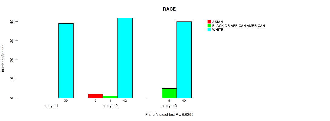
Clustering Approach #4: 'RPPA cHierClus subtypes'

Table S46. Description of clustering approach #4: 'RPPA cHierClus subtypes'

Cluster Labels	1	2	3
Number of samples	48	65	46

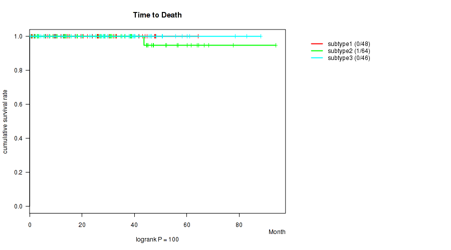
'RPPA cHierClus subtypes' versus 'Time to Death'

P value = 100 (logrank test), Q value = 1

Table S47. Clustering Approach #4: 'RPPA cHierClus subtypes' versus Clinical Feature #1: 'Time to Death'

	nPatients	nDeath	Duration Range (Median), Month
ALL	158	1	0.3 - 94.0 (27.0)
subtype1	48	0	0.7 - 64.5 (20.1)
subtype2	64	1	0.8 - 94.0 (27.9)
subtype3	46	0	0.3 - 88.2 (29.4)

Figure S43. Get High-res Image Clustering Approach #4: 'RPPA cHierClus subtypes' versus Clinical Feature #1: 'Time to Death'

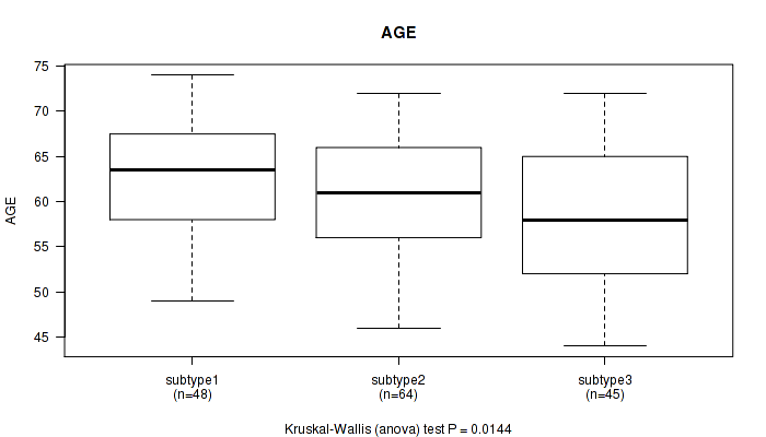
'RPPA cHierClus subtypes' versus 'AGE'

P value = 0.0144 (Kruskal-Wallis (anova)), Q value = 1

Table S48. Clustering Approach #4: 'RPPA cHierClus subtypes' versus Clinical Feature #2: 'AGE'

	nPatients	Mean (Std.Dev)
ALL	157	60.6 (7.1)
subtype1	48	63.0 (6.2)
subtype2	64	60.4 (6.7)
subtype3	45	58.2 (7.8)

Figure S44. Get High-res Image Clustering Approach #4: 'RPPA cHierClus subtypes' versus Clinical Feature #2: 'AGE'

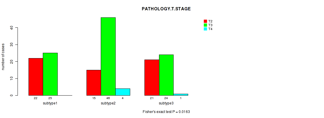
'RPPA cHierClus subtypes' versus 'PATHOLOGY.T.STAGE'

P value = 0.0163 (Fisher's exact test), Q value = 1

Table S49. Clustering Approach #4: 'RPPA cHierClus subtypes' versus Clinical Feature #3: 'PATHOLOGY.T.STAGE'

nPatients	T2	T3	T4
ALL	58	95	5
subtype1	22	25	0
subtype2	15	46	4
subtype3	21	24	1

Figure S45. Get High-res Image Clustering Approach #4: 'RPPA cHierClus subtypes' versus Clinical Feature #3: 'PATHOLOGY.T.STAGE'

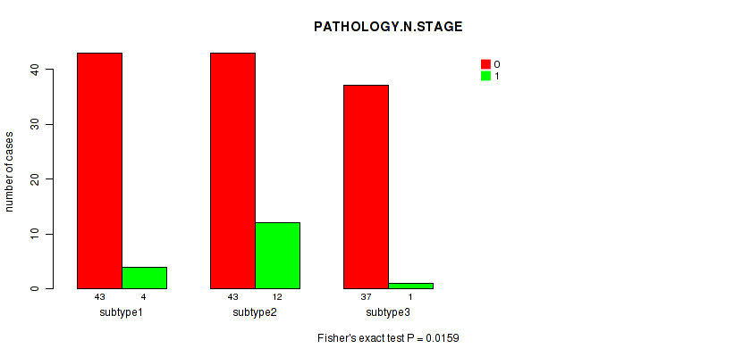
'RPPA cHierClus subtypes' versus 'PATHOLOGY.N.STAGE'

P value = 0.0159 (Fisher's exact test), Q value = 1

Table S50. Clustering Approach #4: 'RPPA cHierClus subtypes' versus Clinical Feature #4: 'PATHOLOGY.N.STAGE'

nPatients	0	1
ALL	123	17
subtype1	43	4
subtype2	43	12
subtype3	37	1

Figure S46. Get High-res Image Clustering Approach #4: 'RPPA cHierClus subtypes' versus Clinical Feature #4: 'PATHOLOGY.N.STAGE'

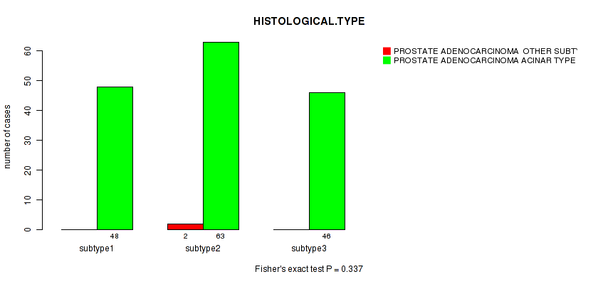
'RPPA cHierClus subtypes' versus 'HISTOLOGICAL.TYPE'

P value = 0.337 (Fisher's exact test), Q value = 1

Table S51. Clustering Approach #4: 'RPPA cHierClus subtypes' versus Clinical Feature #5: 'HISTOLOGICAL.TYPE'

nPatients	PROSTATE ADENOCARCINOMA OTHER SUBTYPE	PROSTATE ADENOCARCINOMA ACINAR TYPE
ALL	2	157
subtype1	0	48
subtype2	2	63
subtype3	0	46

Figure S47. Get High-res Image Clustering Approach #4: 'RPPA cHierClus subtypes' versus Clinical Feature #5: 'HISTOLOGICAL.TYPE'

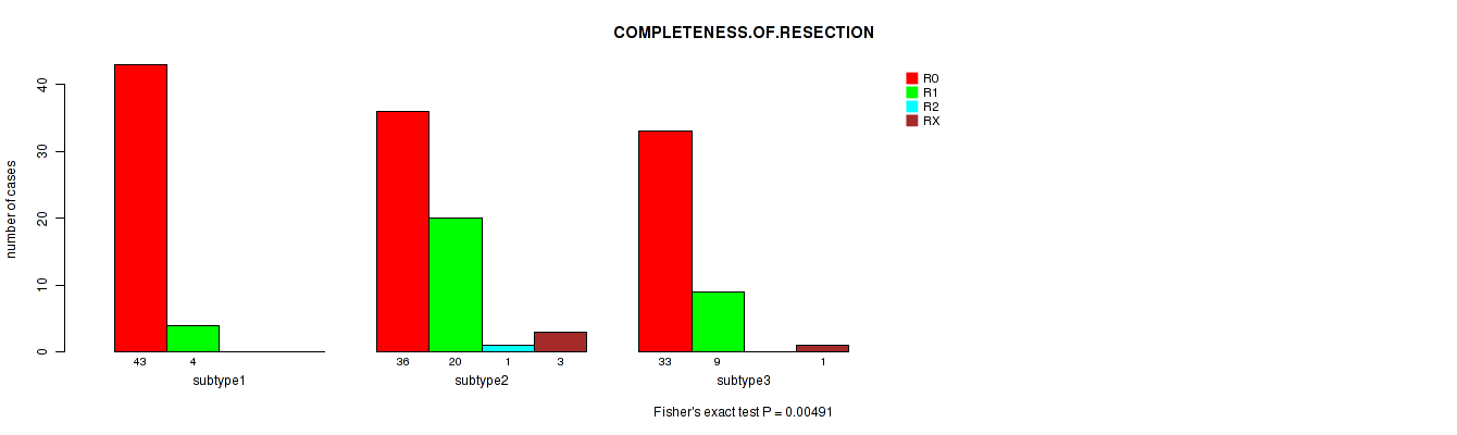
'RPPA cHierClus subtypes' versus 'COMPLETENESS.OF.RESECTION'

P value = 0.00491 (Fisher's exact test), Q value = 0.48

Table S52. Clustering Approach #4: 'RPPA cHierClus subtypes' versus Clinical Feature #6: 'COMPLETENESS.OF.RESECTION'

nPatients	R0	R1	R2	RX
ALL	112	33	1	4
subtype1	43	4	0	0
subtype2	36	20	1	3
subtype3	33	9	0	1

Figure S48. Get High-res Image Clustering Approach #4: 'RPPA cHierClus subtypes' versus Clinical Feature #6: 'COMPLETENESS.OF.RESECTION'

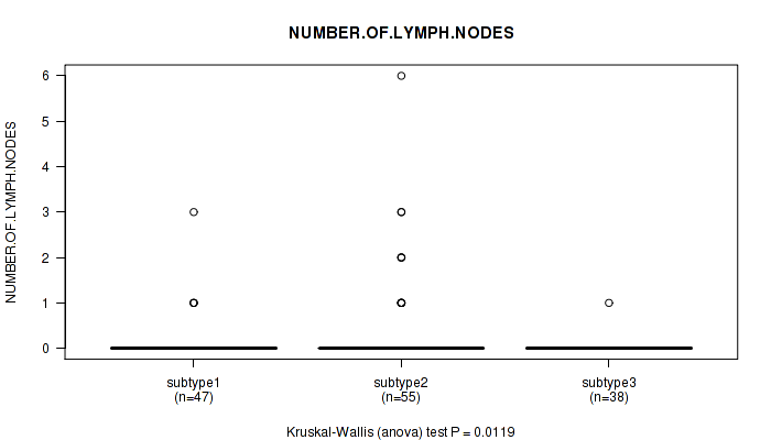
'RPPA cHierClus subtypes' versus 'NUMBER.OF.LYMPH.NODES'

P value = 0.0119 (Kruskal-Wallis (anova)), Q value = 1

Table S53. Clustering Approach #4: 'RPPA cHierClus subtypes' versus Clinical Feature #7: 'NUMBER.OF.LYMPH.NODES'

	nPatients	Mean (Std.Dev)
ALL	140	0.2 (0.7)
subtype1	47	0.1 (0.5)
subtype2	55	0.4 (1.1)
subtype3	38	0.0 (0.2)

Figure S49. Get High-res Image Clustering Approach #4: 'RPPA cHierClus subtypes' versus Clinical Feature #7: 'NUMBER.OF.LYMPH.NODES'

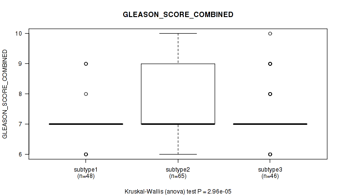
'RPPA cHierClus subtypes' versus 'GLEASON_SCORE_COMBINED'

P value = 2.96e-05 (Kruskal-Wallis (anova)), Q value = 0.0037

Table S54. Clustering Approach #4: 'RPPA cHierClus subtypes' versus Clinical Feature #8: 'GLEASON_SCORE_COMBINED'

	nPatients	Mean (Std.Dev)
ALL	159	7.4 (0.9)
subtype1	48	7.0 (0.5)
subtype2	65	7.8 (1.0)
subtype3	46	7.3 (0.9)

Figure S50. Get High-res Image Clustering Approach #4: 'RPPA cHierClus subtypes' versus Clinical Feature #8: 'GLEASON_SCORE_COMBINED'

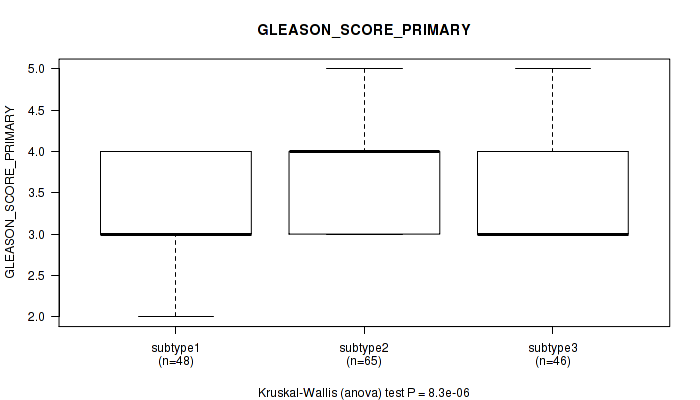
'RPPA cHierClus subtypes' versus 'GLEASON_SCORE_PRIMARY'

P value = 8.3e-06 (Kruskal-Wallis (anova)), Q value = 0.0011

Table S55. Clustering Approach #4: 'RPPA cHierClus subtypes' versus Clinical Feature #9: 'GLEASON_SCORE_PRIMARY'

	nPatients	Mean (Std.Dev)
ALL	159	3.5 (0.6)
subtype1	48	3.4 (0.5)
subtype2	65	3.8 (0.6)
subtype3	46	3.4 (0.5)

Figure S51. Get High-res Image Clustering Approach #4: 'RPPA cHierClus subtypes' versus Clinical Feature #9: 'GLEASON_SCORE_PRIMARY'

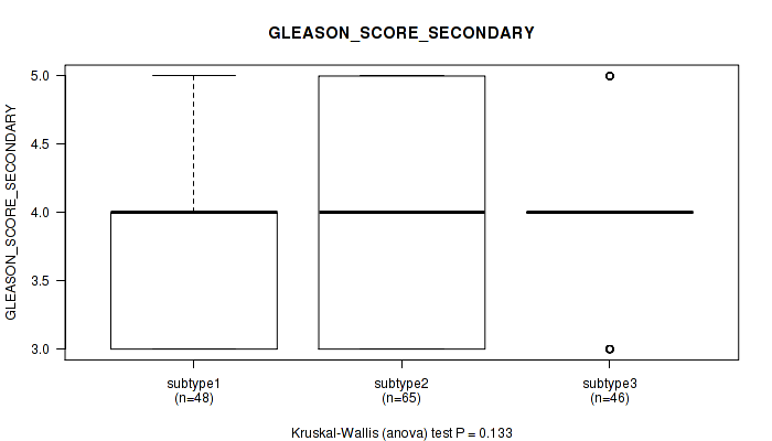
'RPPA cHierClus subtypes' versus 'GLEASON_SCORE_SECONDARY'

P value = 0.133 (Kruskal-Wallis (anova)), Q value = 1

Table S56. Clustering Approach #4: 'RPPA cHierClus subtypes' versus Clinical Feature #10: 'GLEASON_SCORE_SECONDARY'

	nPatients	Mean (Std.Dev)
ALL	159	3.9 (0.7)
subtype1	48	3.7 (0.6)
subtype2	65	4.0 (0.8)
subtype3	46	3.9 (0.6)

Figure S52. Get High-res Image Clustering Approach #4: 'RPPA cHierClus subtypes' versus Clinical Feature #10: 'GLEASON_SCORE_SECONDARY'

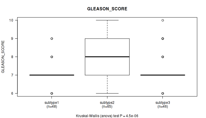
'RPPA cHierClus subtypes' versus 'GLEASON_SCORE'

P value = 4.5e-06 (Kruskal-Wallis (anova)), Q value = 6e-04

Table S57. Clustering Approach #4: 'RPPA cHierClus subtypes' versus Clinical Feature #11: 'GLEASON_SCORE'

	nPatients	Mean (Std.Dev)
ALL	159	7.5 (0.9)
subtype1	48	7.1 (0.6)
subtype2	65	7.9 (1.0)
subtype3	46	7.3 (0.9)

Figure S53. Get High-res Image Clustering Approach #4: 'RPPA cHierClus subtypes' versus Clinical Feature #11: 'GLEASON_SCORE'

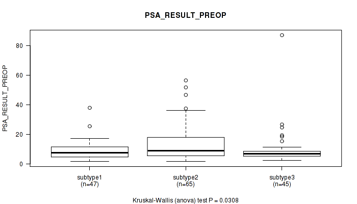
'RPPA cHierClus subtypes' versus 'PSA_RESULT_PREOP'

P value = 0.0308 (Kruskal-Wallis (anova)), Q value = 1

Table S58. Clustering Approach #4: 'RPPA cHierClus subtypes' versus Clinical Feature #12: 'PSA_RESULT_PREOP'

	nPatients	Mean (Std.Dev)
ALL	157	11.2 (11.2)
subtype1	47	8.9 (6.4)
subtype2	65	14.0 (12.2)
subtype3	45	9.7 (12.9)

Figure S54. Get High-res Image Clustering Approach #4: 'RPPA cHierClus subtypes' versus Clinical Feature #12: 'PSA_RESULT_PREOP'

'RPPA cHierClus subtypes' versus 'PSA_VALUE'

P value = 0.494 (Kruskal-Wallis (anova)), Q value = 1

Table S59. Clustering Approach #4: 'RPPA cHierClus subtypes' versus Clinical Feature #13: 'PSA_VALUE'

	nPatients	Mean (Std.Dev)
ALL	144	1.4 (4.4)
subtype1	47	1.4 (3.7)
subtype2	56	2.0 (5.7)
subtype3	41	0.6 (3.1)

Figure S55. Get High-res Image Clustering Approach #4: 'RPPA cHierClus subtypes' versus Clinical Feature #13: 'PSA_VALUE'

'RPPA cHierClus subtypes' versus 'RACE'

P value = 0.00843 (Fisher's exact test), Q value = 0.75

Table S60. Clustering Approach #4: 'RPPA cHierClus subtypes' versus Clinical Feature #14: 'RACE'

nPatients	ASIAN	BLACK OR AFRICAN AMERICAN	WHITE
ALL	2	6	121
subtype1	0	0	45
subtype2	0	5	40
subtype3	2	1	36

Figure S56. Get High-res Image Clustering Approach #4: 'RPPA cHierClus subtypes' versus Clinical Feature #14: 'RACE'

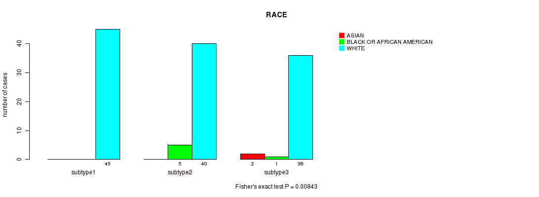
Clustering Approach #5: 'RNAseq CNMF subtypes'

Table S61. Description of clustering approach #5: 'RNAseq CNMF subtypes'

Cluster Labels	1	2	3
Number of samples	107	123	130

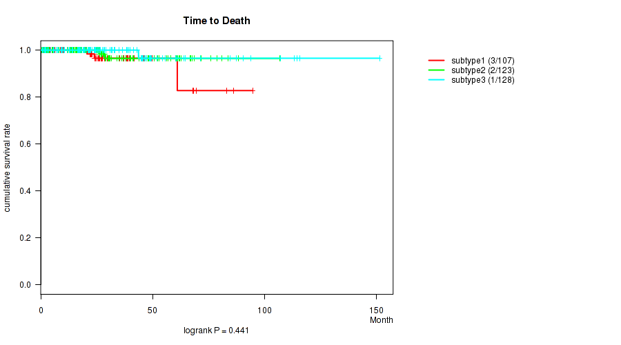
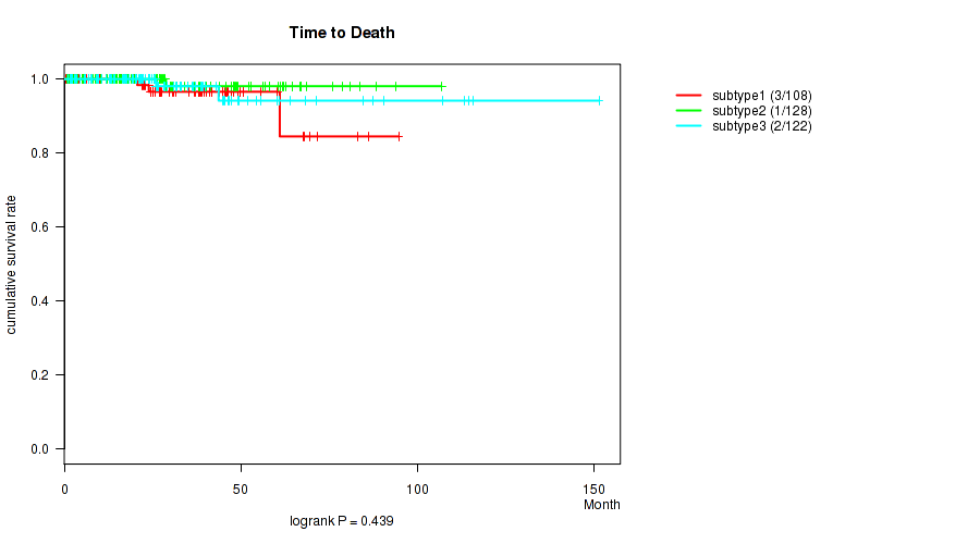
'RNAseq CNMF subtypes' versus 'Time to Death'

P value = 0.441 (logrank test), Q value = 1

Table S62. Clustering Approach #5: 'RNAseq CNMF subtypes' versus Clinical Feature #1: 'Time to Death'

	nPatients	nDeath	Duration Range (Median), Month
ALL	358	6	0.3 - 151.4 (23.9)
subtype1	107	3	0.7 - 94.7 (24.0)
subtype2	123	2	0.3 - 106.8 (25.5)
subtype3	128	1	0.8 - 151.4 (22.2)

Figure S57. Get High-res Image Clustering Approach #5: 'RNAseq CNMF subtypes' versus Clinical Feature #1: 'Time to Death'

'RNAseq CNMF subtypes' versus 'AGE'

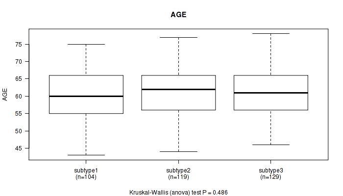
P value = 0.486 (Kruskal-Wallis (anova)), Q value = 1

Table S63. Clustering Approach #5: 'RNAseq CNMF subtypes' versus Clinical Feature #2: 'AGE'

	nPatients	Mean (Std.Dev)
ALL	352	60.7 (6.9)
subtype1	104	60.0 (7.2)
subtype2	119	61.1 (6.9)
subtype3	129	61.0 (6.8)

Figure S58. Get High-res Image Clustering Approach #5: 'RNAseq CNMF subtypes' versus Clinical Feature #2: 'AGE'

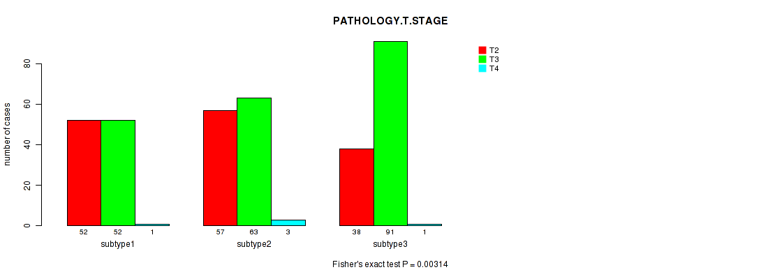
'RNAseq CNMF subtypes' versus 'PATHOLOGY.T.STAGE'

P value = 0.00314 (Fisher's exact test), Q value = 0.32

Table S64. Clustering Approach #5: 'RNAseq CNMF subtypes' versus Clinical Feature #3: 'PATHOLOGY.T.STAGE'

nPatients	T2	T3	T4
ALL	147	206	5
subtype1	52	52	1
subtype2	57	63	3
subtype3	38	91	1

Figure S59. Get High-res Image Clustering Approach #5: 'RNAseq CNMF subtypes' versus Clinical Feature #3: 'PATHOLOGY.T.STAGE'

'RNAseq CNMF subtypes' versus 'PATHOLOGY.N.STAGE'

P value = 0.127 (Fisher's exact test), Q value = 1

Table S65. Clustering Approach #5: 'RNAseq CNMF subtypes' versus Clinical Feature #4: 'PATHOLOGY.N.STAGE'

nPatients	0	1
ALL	260	45
subtype1	80	8
subtype2	88	15
subtype3	92	22

Figure S60. Get High-res Image Clustering Approach #5: 'RNAseq CNMF subtypes' versus Clinical Feature #4: 'PATHOLOGY.N.STAGE'

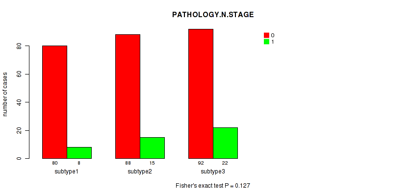
'RNAseq CNMF subtypes' versus 'HISTOLOGICAL.TYPE'

P value = 0.683 (Fisher's exact test), Q value = 1

Table S66. Clustering Approach #5: 'RNAseq CNMF subtypes' versus Clinical Feature #5: 'HISTOLOGICAL.TYPE'

nPatients	PROSTATE ADENOCARCINOMA OTHER SUBTYPE	PROSTATE ADENOCARCINOMA ACINAR TYPE
ALL	13	347
subtype1	4	103
subtype2	3	120
subtype3	6	124

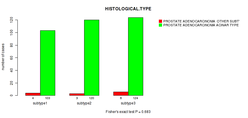
Figure S61. Get High-res Image Clustering Approach #5: 'RNAseq CNMF subtypes' versus Clinical Feature #5: 'HISTOLOGICAL.TYPE'

'RNAseq CNMF subtypes' versus 'COMPLETENESS.OF.RESECTION'

P value = 0.446 (Fisher's exact test), Q value = 1

Table S67. Clustering Approach #5: 'RNAseq CNMF subtypes' versus Clinical Feature #6: 'COMPLETENESS.OF.RESECTION'

nPatients	R0	R1	R2	RX
ALL	242	89	5	10
subtype1	77	21	0	3
subtype2	77	37	2	3
subtype3	88	31	3	4

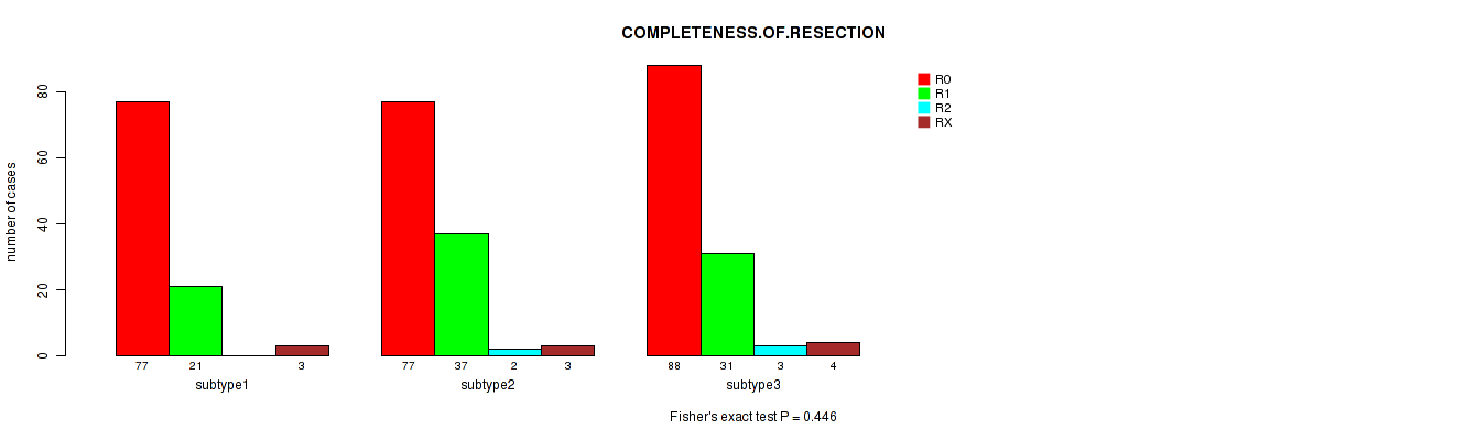
Figure S62. Get High-res Image Clustering Approach #5: 'RNAseq CNMF subtypes' versus Clinical Feature #6: 'COMPLETENESS.OF.RESECTION'

'RNAseq CNMF subtypes' versus 'NUMBER.OF.LYMPH.NODES'

P value = 0.104 (Kruskal-Wallis (anova)), Q value = 1

Table S68. Clustering Approach #5: 'RNAseq CNMF subtypes' versus Clinical Feature #7: 'NUMBER.OF.LYMPH.NODES'

	nPatients	Mean (Std.Dev)
ALL	301	0.3 (1.3)
subtype1	86	0.1 (0.5)
subtype2	101	0.3 (0.9)
subtype3	114	0.6 (1.9)

Figure S63. Get High-res Image Clustering Approach #5: 'RNAseq CNMF subtypes' versus Clinical Feature #7: 'NUMBER.OF.LYMPH.NODES'

'RNAseq CNMF subtypes' versus 'GLEASON_SCORE_COMBINED'

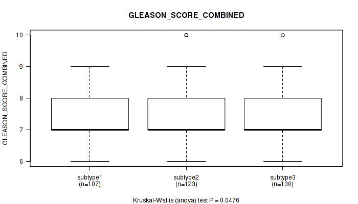
P value = 0.0476 (Kruskal-Wallis (anova)), Q value = 1

Table S69. Clustering Approach #5: 'RNAseq CNMF subtypes' versus Clinical Feature #8: 'GLEASON_SCORE_COMBINED'

	nPatients	Mean (Std.Dev)
ALL	360	7.4 (0.9)
subtype1	107	7.3 (0.8)
subtype2	123	7.4 (1.0)
subtype3	130	7.6 (0.9)

Figure S64. Get High-res Image Clustering Approach #5: 'RNAseq CNMF subtypes' versus Clinical Feature #8: 'GLEASON_SCORE_COMBINED'

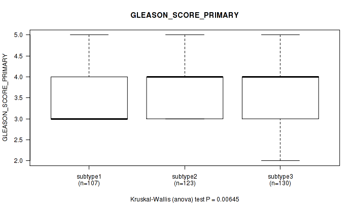
'RNAseq CNMF subtypes' versus 'GLEASON_SCORE_PRIMARY'

P value = 0.00645 (Kruskal-Wallis (anova)), Q value = 0.6

Table S70. Clustering Approach #5: 'RNAseq CNMF subtypes' versus Clinical Feature #9: 'GLEASON_SCORE_PRIMARY'

	nPatients	Mean (Std.Dev)
ALL	360	3.6 (0.6)
subtype1	107	3.4 (0.6)
subtype2	123	3.7 (0.6)
subtype3	130	3.7 (0.6)

Figure S65. Get High-res Image Clustering Approach #5: 'RNAseq CNMF subtypes' versus Clinical Feature #9: 'GLEASON_SCORE_PRIMARY'

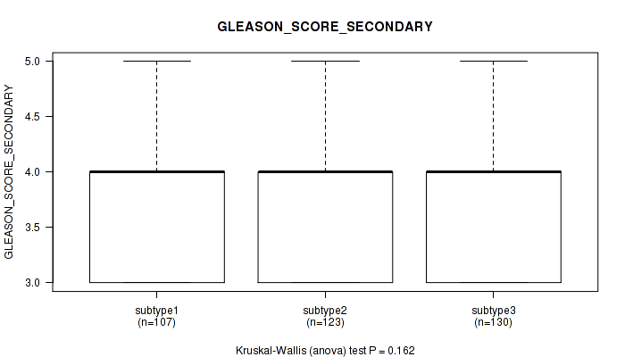
'RNAseq CNMF subtypes' versus 'GLEASON_SCORE_SECONDARY'

P value = 0.162 (Kruskal-Wallis (anova)), Q value = 1

Table S71. Clustering Approach #5: 'RNAseq CNMF subtypes' versus Clinical Feature #10: 'GLEASON_SCORE_SECONDARY'

	nPatients	Mean (Std.Dev)
ALL	360	3.8 (0.6)
subtype1	107	3.8 (0.6)
subtype2	123	3.8 (0.7)
subtype3	130	3.9 (0.7)

Figure S66. Get High-res Image Clustering Approach #5: 'RNAseq CNMF subtypes' versus Clinical Feature #10: 'GLEASON_SCORE_SECONDARY'

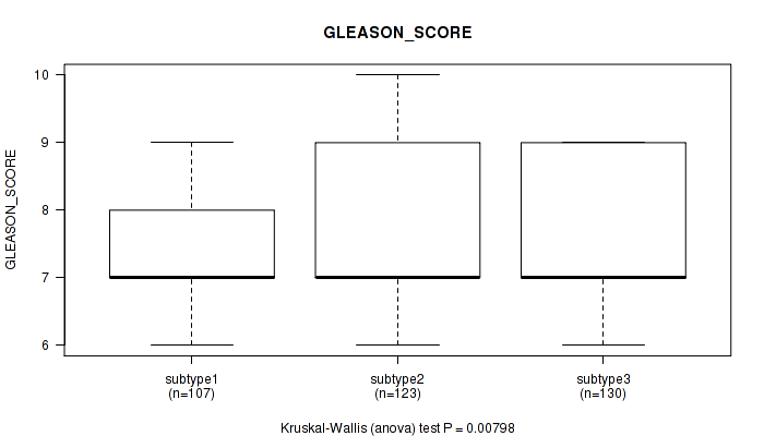
'RNAseq CNMF subtypes' versus 'GLEASON_SCORE'

P value = 0.00798 (Kruskal-Wallis (anova)), Q value = 0.72

Table S72. Clustering Approach #5: 'RNAseq CNMF subtypes' versus Clinical Feature #11: 'GLEASON_SCORE'

	nPatients	Mean (Std.Dev)
ALL	360	7.5 (1.0)
subtype1	107	7.3 (0.8)
subtype2	123	7.6 (1.0)
subtype3	130	7.7 (0.9)

Figure S67. Get High-res Image Clustering Approach #5: 'RNAseq CNMF subtypes' versus Clinical Feature #11: 'GLEASON_SCORE'

'RNAseq CNMF subtypes' versus 'PSA_RESULT_PREOP'

P value = 0.00327 (Kruskal-Wallis (anova)), Q value = 0.33

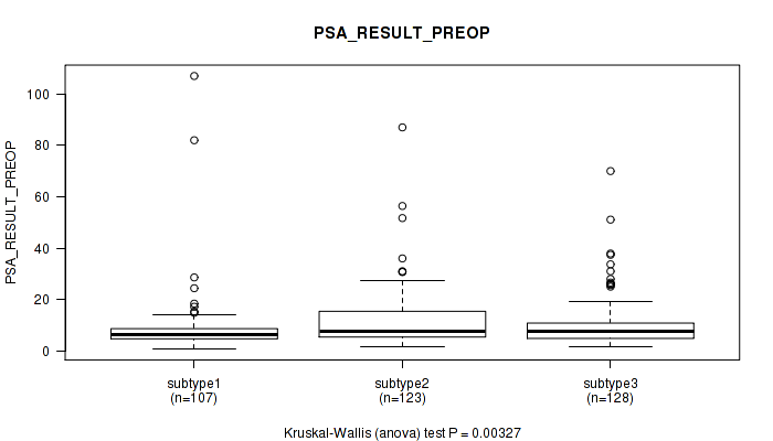
Table S73. Clustering Approach #5: 'RNAseq CNMF subtypes' versus Clinical Feature #12: 'PSA_RESULT_PREOP'

	nPatients	Mean (Std.Dev)
ALL	358	10.5 (11.3)
subtype1	107	8.9 (12.7)
subtype2	123	12.2 (11.6)
subtype3	128	10.3 (9.6)

Figure S68. Get High-res Image Clustering Approach #5: 'RNAseq CNMF subtypes' versus Clinical Feature #12: 'PSA_RESULT_PREOP'

'RNAseq CNMF subtypes' versus 'PSA_VALUE'

P value = 0.114 (Kruskal-Wallis (anova)), Q value = 1

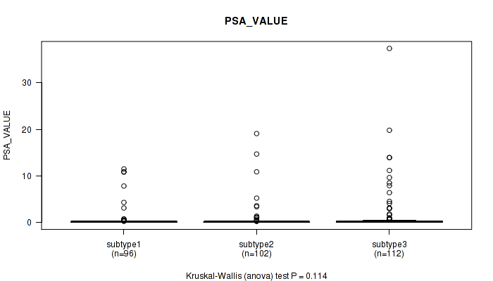
Table S74. Clustering Approach #5: 'RNAseq CNMF subtypes' versus Clinical Feature #13: 'PSA_VALUE'

	nPatients	Mean (Std.Dev)
ALL	310	0.9 (3.4)
subtype1	96	0.6 (2.1)
subtype2	102	0.7 (2.6)
subtype3	112	1.5 (4.7)

Figure S69. Get High-res Image Clustering Approach #5: 'RNAseq CNMF subtypes' versus Clinical Feature #13: 'PSA_VALUE'

'RNAseq CNMF subtypes' versus 'RACE'

P value = 0.0702 (Fisher's exact test), Q value = 1

Table S75. Clustering Approach #5: 'RNAseq CNMF subtypes' versus Clinical Feature #14: 'RACE'

nPatients	ASIAN	BLACK OR AFRICAN AMERICAN	WHITE
ALL	2	7	147
subtype1	2	0	52
subtype2	0	3	40
subtype3	0	4	55

Figure S70. Get High-res Image Clustering Approach #5: 'RNAseq CNMF subtypes' versus Clinical Feature #14: 'RACE'

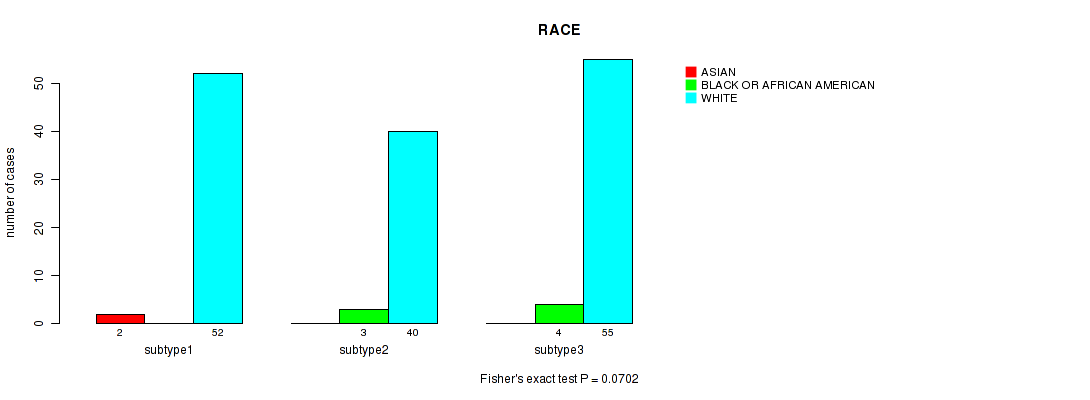
Clustering Approach #6: 'RNAseq cHierClus subtypes'

Table S76. Description of clustering approach #6: 'RNAseq cHierClus subtypes'

Cluster Labels	1	2	3
Number of samples	108	128	124

'RNAseq cHierClus subtypes' versus 'Time to Death'

P value = 0.439 (logrank test), Q value = 1

Table S77. Clustering Approach #6: 'RNAseq cHierClus subtypes' versus Clinical Feature #1: 'Time to Death'

	nPatients	nDeath	Duration Range (Median), Month
ALL	358	6	0.3 - 151.4 (23.9)
subtype1	108	3	0.3 - 94.7 (24.2)
subtype2	128	1	0.8 - 106.8 (25.4)
subtype3	122	2	1.0 - 151.4 (22.7)

Figure S71. Get High-res Image Clustering Approach #6: 'RNAseq cHierClus subtypes' versus Clinical Feature #1: 'Time to Death'

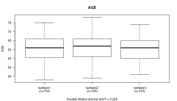
'RNAseq cHierClus subtypes' versus 'AGE'

P value = 0.226 (Kruskal-Wallis (anova)), Q value = 1

Table S78. Clustering Approach #6: 'RNAseq cHierClus subtypes' versus Clinical Feature #2: 'AGE'

	nPatients	Mean (Std.Dev)
ALL	352	60.7 (6.9)
subtype1	103	60.7 (6.9)
subtype2	126	61.5 (7.2)
subtype3	123	59.9 (6.6)

Figure S72. Get High-res Image Clustering Approach #6: 'RNAseq cHierClus subtypes' versus Clinical Feature #2: 'AGE'

'RNAseq cHierClus subtypes' versus 'PATHOLOGY.T.STAGE'

P value = 0.0201 (Fisher's exact test), Q value = 1

Table S79. Clustering Approach #6: 'RNAseq cHierClus subtypes' versus Clinical Feature #3: 'PATHOLOGY.T.STAGE'

nPatients	T2	T3	T4
ALL	147	206	5
subtype1	55	50	1
subtype2	52	73	3
subtype3	40	83	1

Figure S73. Get High-res Image Clustering Approach #6: 'RNAseq cHierClus subtypes' versus Clinical Feature #3: 'PATHOLOGY.T.STAGE'

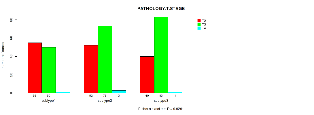
'RNAseq cHierClus subtypes' versus 'PATHOLOGY.N.STAGE'

P value = 0.0377 (Fisher's exact test), Q value = 1

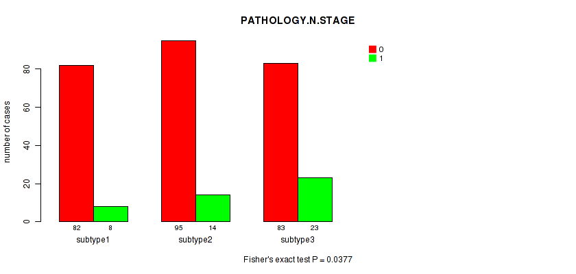
Table S80. Clustering Approach #6: 'RNAseq cHierClus subtypes' versus Clinical Feature #4: 'PATHOLOGY.N.STAGE'

nPatients	0	1
ALL	260	45
subtype1	82	8
subtype2	95	14
subtype3	83	23

Figure S74. Get High-res Image Clustering Approach #6: 'RNAseq cHierClus subtypes' versus Clinical Feature #4: 'PATHOLOGY.N.STAGE'

'RNAseq cHierClus subtypes' versus 'HISTOLOGICAL.TYPE'

P value = 0.94 (Fisher's exact test), Q value = 1

Table S81. Clustering Approach #6: 'RNAseq cHierClus subtypes' versus Clinical Feature #5: 'HISTOLOGICAL.TYPE'

nPatients	PROSTATE ADENOCARCINOMA OTHER SUBTYPE	PROSTATE ADENOCARCINOMA ACINAR TYPE
ALL	13	347
subtype1	4	104
subtype2	4	124
subtype3	5	119

Figure S75. Get High-res Image Clustering Approach #6: 'RNAseq cHierClus subtypes' versus Clinical Feature #5: 'HISTOLOGICAL.TYPE'

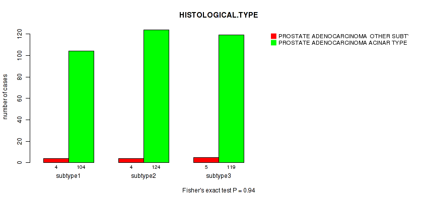
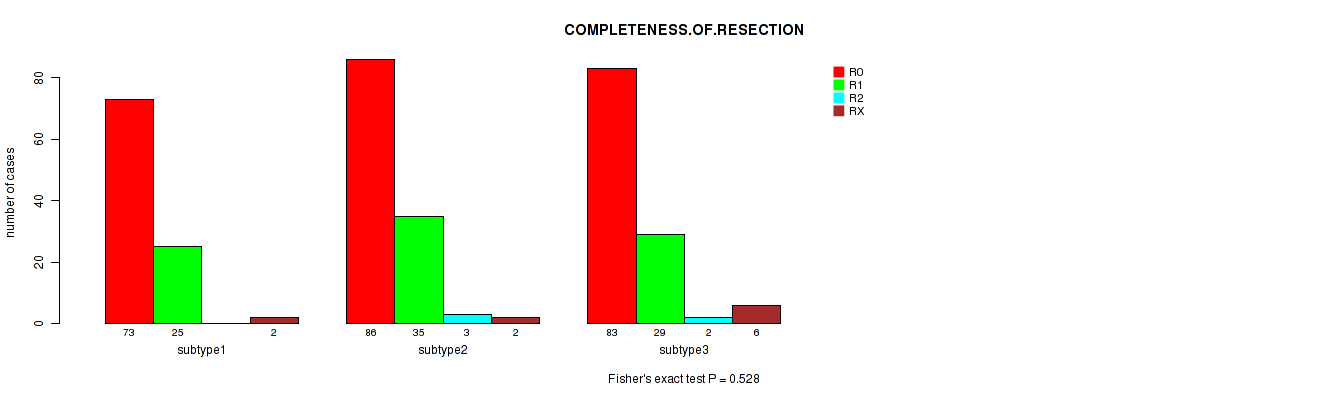
'RNAseq cHierClus subtypes' versus 'COMPLETENESS.OF.RESECTION'

P value = 0.528 (Fisher's exact test), Q value = 1

Table S82. Clustering Approach #6: 'RNAseq cHierClus subtypes' versus Clinical Feature #6: 'COMPLETENESS.OF.RESECTION'

nPatients	R0	R1	R2	RX
ALL	242	89	5	10
subtype1	73	25	0	2
subtype2	86	35	3	2
subtype3	83	29	2	6

Figure S76. Get High-res Image Clustering Approach #6: 'RNAseq cHierClus subtypes' versus Clinical Feature #6: 'COMPLETENESS.OF.RESECTION'

'RNAseq cHierClus subtypes' versus 'NUMBER.OF.LYMPH.NODES'

P value = 0.0268 (Kruskal-Wallis (anova)), Q value = 1

Table S83. Clustering Approach #6: 'RNAseq cHierClus subtypes' versus Clinical Feature #7: 'NUMBER.OF.LYMPH.NODES'

	nPatients	Mean (Std.Dev)
ALL	301	0.3 (1.3)
subtype1	87	0.1 (0.5)
subtype2	108	0.2 (0.8)
subtype3	106	0.7 (2.0)

Figure S77. Get High-res Image Clustering Approach #6: 'RNAseq cHierClus subtypes' versus Clinical Feature #7: 'NUMBER.OF.LYMPH.NODES'

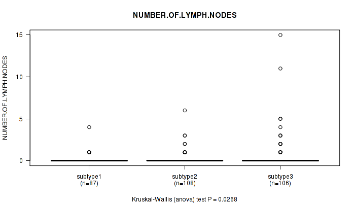
'RNAseq cHierClus subtypes' versus 'GLEASON_SCORE_COMBINED'

P value = 0.0215 (Kruskal-Wallis (anova)), Q value = 1

Table S84. Clustering Approach #6: 'RNAseq cHierClus subtypes' versus Clinical Feature #8: 'GLEASON_SCORE_COMBINED'

	nPatients	Mean (Std.Dev)
ALL	360	7.4 (0.9)
subtype1	108	7.2 (0.8)
subtype2	128	7.5 (1.0)
subtype3	124	7.5 (1.0)

Figure S78. Get High-res Image Clustering Approach #6: 'RNAseq cHierClus subtypes' versus Clinical Feature #8: 'GLEASON_SCORE_COMBINED'

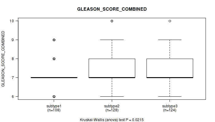
'RNAseq cHierClus subtypes' versus 'GLEASON_SCORE_PRIMARY'

P value = 0.00463 (Kruskal-Wallis (anova)), Q value = 0.46

Table S85. Clustering Approach #6: 'RNAseq cHierClus subtypes' versus Clinical Feature #9: 'GLEASON_SCORE_PRIMARY'

	nPatients	Mean (Std.Dev)
ALL	360	3.6 (0.6)
subtype1	108	3.5 (0.6)
subtype2	128	3.7 (0.6)
subtype3	124	3.6 (0.6)

Figure S79. Get High-res Image Clustering Approach #6: 'RNAseq cHierClus subtypes' versus Clinical Feature #9: 'GLEASON_SCORE_PRIMARY'

'RNAseq cHierClus subtypes' versus 'GLEASON_SCORE_SECONDARY'

P value = 0.262 (Kruskal-Wallis (anova)), Q value = 1

Table S86. Clustering Approach #6: 'RNAseq cHierClus subtypes' versus Clinical Feature #10: 'GLEASON_SCORE_SECONDARY'

	nPatients	Mean (Std.Dev)
ALL	360	3.8 (0.6)
subtype1	108	3.8 (0.6)
subtype2	128	3.8 (0.7)
subtype3	124	3.9 (0.7)

Figure S80. Get High-res Image Clustering Approach #6: 'RNAseq cHierClus subtypes' versus Clinical Feature #10: 'GLEASON_SCORE_SECONDARY'

'RNAseq cHierClus subtypes' versus 'GLEASON_SCORE'

P value = 0.00552 (Kruskal-Wallis (anova)), Q value = 0.52

Table S87. Clustering Approach #6: 'RNAseq cHierClus subtypes' versus Clinical Feature #11: 'GLEASON_SCORE'

	nPatients	Mean (Std.Dev)
ALL	360	7.5 (1.0)
subtype1	108	7.3 (0.8)
subtype2	128	7.6 (1.0)
subtype3	124	7.6 (1.0)

Figure S81. Get High-res Image Clustering Approach #6: 'RNAseq cHierClus subtypes' versus Clinical Feature #11: 'GLEASON_SCORE'

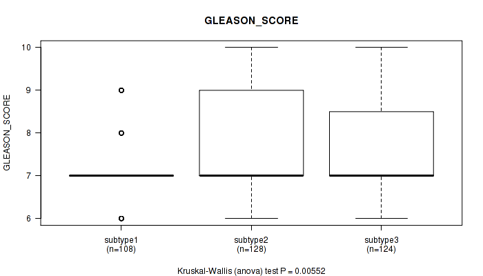
'RNAseq cHierClus subtypes' versus 'PSA_RESULT_PREOP'

P value = 0.00776 (Kruskal-Wallis (anova)), Q value = 0.71

Table S88. Clustering Approach #6: 'RNAseq cHierClus subtypes' versus Clinical Feature #12: 'PSA_RESULT_PREOP'

	nPatients	Mean (Std.Dev)
ALL	358	10.5 (11.3)
subtype1	108	9.2 (12.9)
subtype2	128	12.3 (12.4)
subtype3	122	9.8 (8.1)

Figure S82. Get High-res Image Clustering Approach #6: 'RNAseq cHierClus subtypes' versus Clinical Feature #12: 'PSA_RESULT_PREOP'

'RNAseq cHierClus subtypes' versus 'PSA_VALUE'

P value = 0.31 (Kruskal-Wallis (anova)), Q value = 1

Table S89. Clustering Approach #6: 'RNAseq cHierClus subtypes' versus Clinical Feature #13: 'PSA_VALUE'

	nPatients	Mean (Std.Dev)
ALL	310	0.9 (3.4)
subtype1	93	0.6 (2.1)
subtype2	108	0.8 (2.6)
subtype3	109	1.4 (4.7)

Figure S83. Get High-res Image Clustering Approach #6: 'RNAseq cHierClus subtypes' versus Clinical Feature #13: 'PSA_VALUE'

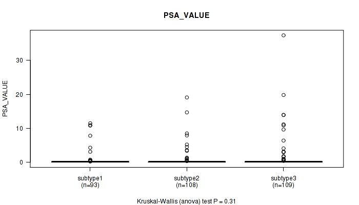
'RNAseq cHierClus subtypes' versus 'RACE'

P value = 0.0656 (Fisher's exact test), Q value = 1

Table S90. Clustering Approach #6: 'RNAseq cHierClus subtypes' versus Clinical Feature #14: 'RACE'

nPatients	ASIAN	BLACK OR AFRICAN AMERICAN	WHITE
ALL	2	7	147
subtype1	1	0	49
subtype2	0	5	42
subtype3	1	2	56

Figure S84. Get High-res Image Clustering Approach #6: 'RNAseq cHierClus subtypes' versus Clinical Feature #14: 'RACE'

Clustering Approach #7: 'MIRSEQ CNMF'

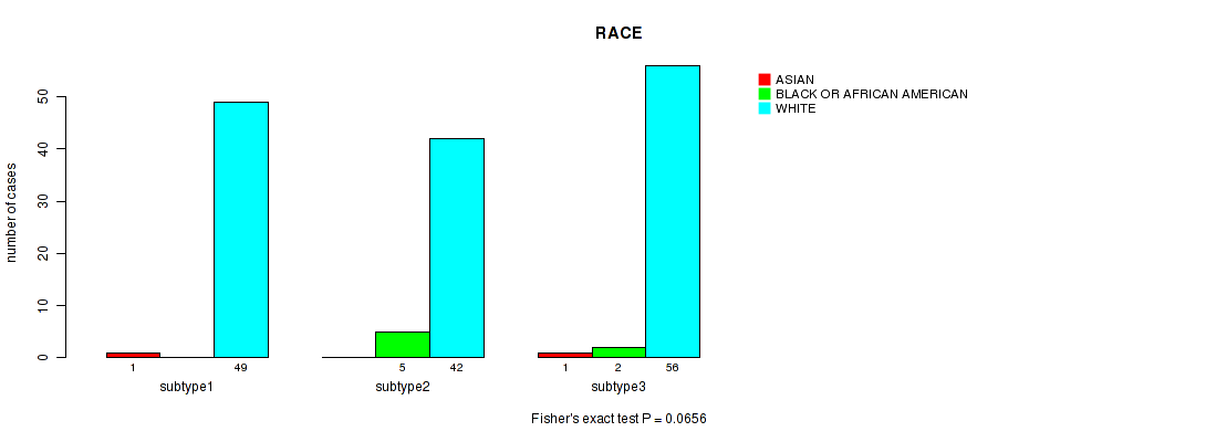
Table S91. Description of clustering approach #7: 'MIRSEQ CNMF'

Cluster Labels	1	2	3
Number of samples	115	116	132

'MIRSEQ CNMF' versus 'Time to Death'

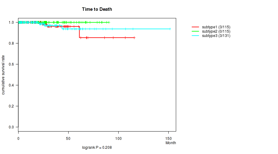
P value = 0.208 (logrank test), Q value = 1

Table S92. Clustering Approach #7: 'MIRSEQ CNMF' versus Clinical Feature #1: 'Time to Death'

	nPatients	nDeath	Duration Range (Median), Month
ALL	361	6	0.3 - 151.4 (23.9)
subtype1	115	3	1.0 - 115.9 (22.4)
subtype2	115	0	0.3 - 90.5 (24.6)
subtype3	131	3	0.8 - 151.4 (24.0)

Figure S85. Get High-res Image Clustering Approach #7: 'MIRSEQ CNMF' versus Clinical Feature #1: 'Time to Death'

'MIRSEQ CNMF' versus 'AGE'

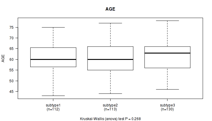
P value = 0.268 (Kruskal-Wallis (anova)), Q value = 1

Table S93. Clustering Approach #7: 'MIRSEQ CNMF' versus Clinical Feature #2: 'AGE'

	nPatients	Mean (Std.Dev)
ALL	355	60.8 (7.0)
subtype1	112	60.4 (6.5)
subtype2	113	60.3 (7.4)
subtype3	130	61.7 (7.0)

Figure S86. Get High-res Image Clustering Approach #7: 'MIRSEQ CNMF' versus Clinical Feature #2: 'AGE'

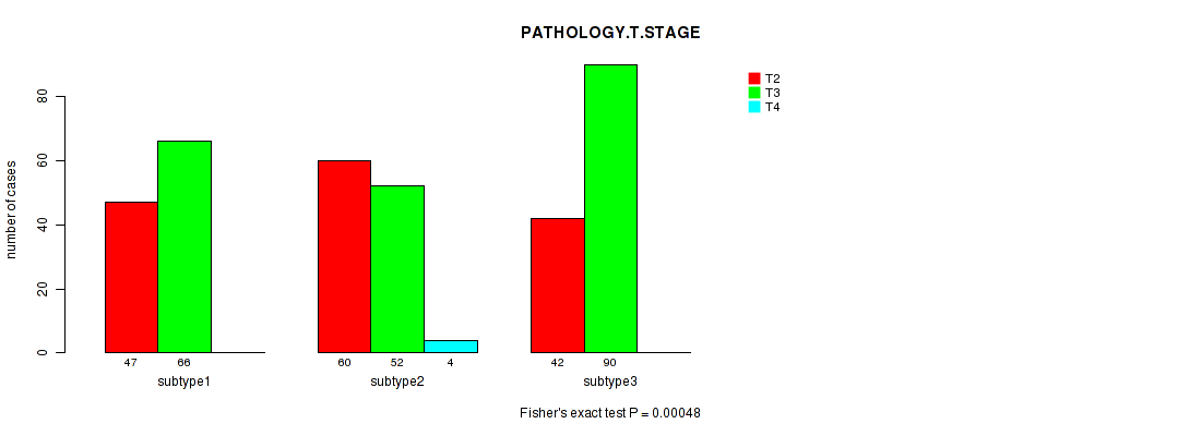
'MIRSEQ CNMF' versus 'PATHOLOGY.T.STAGE'

P value = 0.00048 (Fisher's exact test), Q value = 0.055

Table S94. Clustering Approach #7: 'MIRSEQ CNMF' versus Clinical Feature #3: 'PATHOLOGY.T.STAGE'

nPatients	T2	T3	T4
ALL	149	208	4
subtype1	47	66	0
subtype2	60	52	4
subtype3	42	90	0

Figure S87. Get High-res Image Clustering Approach #7: 'MIRSEQ CNMF' versus Clinical Feature #3: 'PATHOLOGY.T.STAGE'

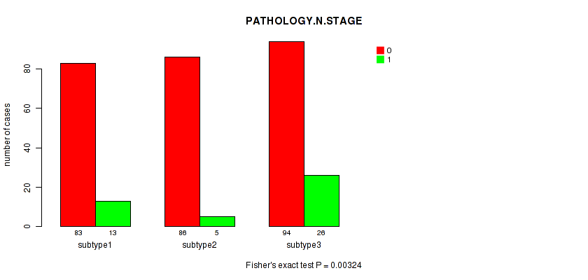
'MIRSEQ CNMF' versus 'PATHOLOGY.N.STAGE'

P value = 0.00324 (Fisher's exact test), Q value = 0.33

Table S95. Clustering Approach #7: 'MIRSEQ CNMF' versus Clinical Feature #4: 'PATHOLOGY.N.STAGE'

nPatients	0	1
ALL	263	44
subtype1	83	13
subtype2	86	5
subtype3	94	26

Figure S88. Get High-res Image Clustering Approach #7: 'MIRSEQ CNMF' versus Clinical Feature #4: 'PATHOLOGY.N.STAGE'

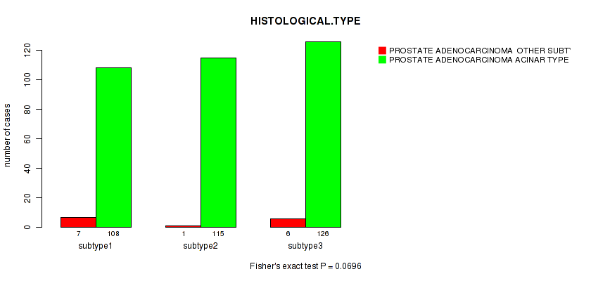
'MIRSEQ CNMF' versus 'HISTOLOGICAL.TYPE'

P value = 0.0696 (Fisher's exact test), Q value = 1

Table S96. Clustering Approach #7: 'MIRSEQ CNMF' versus Clinical Feature #5: 'HISTOLOGICAL.TYPE'

nPatients	PROSTATE ADENOCARCINOMA OTHER SUBTYPE	PROSTATE ADENOCARCINOMA ACINAR TYPE
ALL	14	349
subtype1	7	108
subtype2	1	115
subtype3	6	126

Figure S89. Get High-res Image Clustering Approach #7: 'MIRSEQ CNMF' versus Clinical Feature #5: 'HISTOLOGICAL.TYPE'

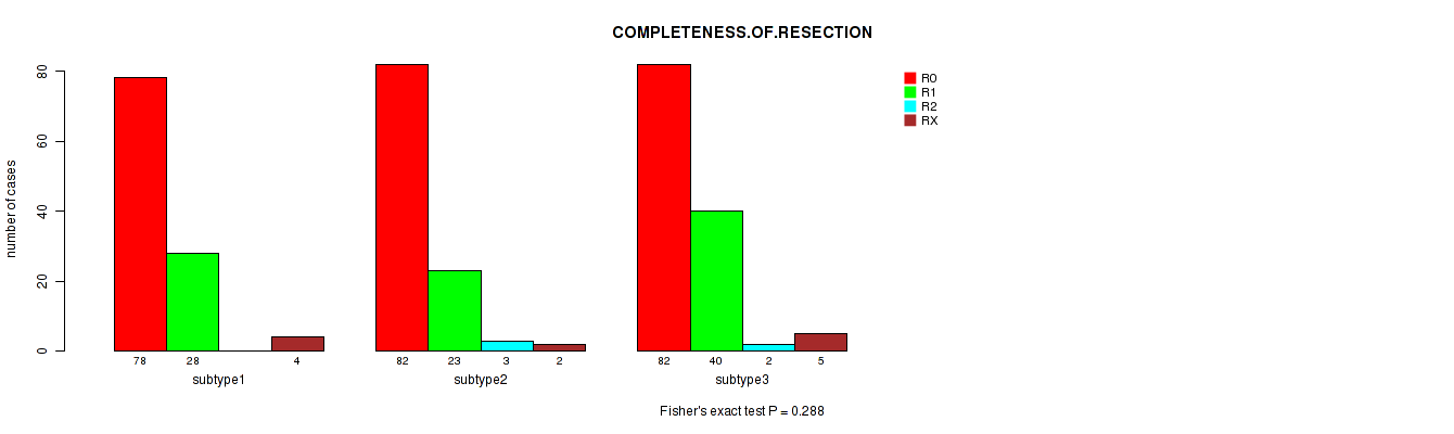
'MIRSEQ CNMF' versus 'COMPLETENESS.OF.RESECTION'

P value = 0.288 (Fisher's exact test), Q value = 1

Table S97. Clustering Approach #7: 'MIRSEQ CNMF' versus Clinical Feature #6: 'COMPLETENESS.OF.RESECTION'

nPatients	R0	R1	R2	RX
ALL	242	91	5	11
subtype1	78	28	0	4
subtype2	82	23	3	2
subtype3	82	40	2	5

Figure S90. Get High-res Image Clustering Approach #7: 'MIRSEQ CNMF' versus Clinical Feature #6: 'COMPLETENESS.OF.RESECTION'

'MIRSEQ CNMF' versus 'NUMBER.OF.LYMPH.NODES'

P value = 0.00216 (Kruskal-Wallis (anova)), Q value = 0.23

Table S98. Clustering Approach #7: 'MIRSEQ CNMF' versus Clinical Feature #7: 'NUMBER.OF.LYMPH.NODES'

	nPatients	Mean (Std.Dev)
ALL	303	0.3 (1.3)
subtype1	93	0.3 (1.3)
subtype2	91	0.1 (0.2)
subtype3	119	0.6 (1.7)

Figure S91. Get High-res Image Clustering Approach #7: 'MIRSEQ CNMF' versus Clinical Feature #7: 'NUMBER.OF.LYMPH.NODES'

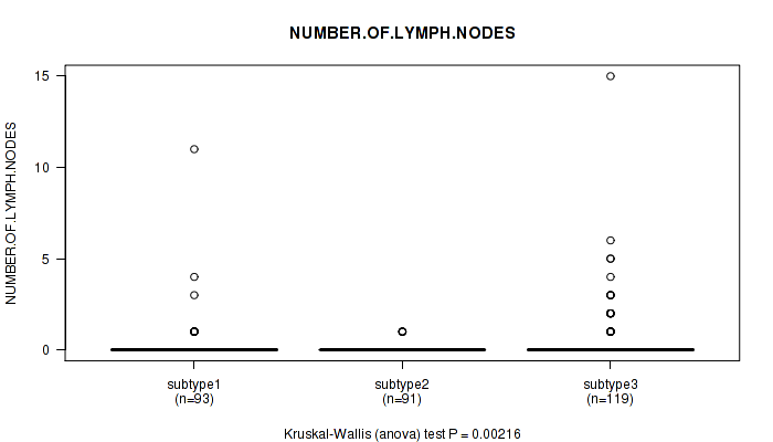
'MIRSEQ CNMF' versus 'GLEASON_SCORE_COMBINED'

P value = 2.91e-06 (Kruskal-Wallis (anova)), Q value = 4e-04

Table S99. Clustering Approach #7: 'MIRSEQ CNMF' versus Clinical Feature #8: 'GLEASON_SCORE_COMBINED'

	nPatients	Mean (Std.Dev)
ALL	363	7.4 (0.9)
subtype1	115	7.4 (0.9)
subtype2	116	7.2 (0.8)
subtype3	132	7.7 (0.9)

Figure S92. Get High-res Image Clustering Approach #7: 'MIRSEQ CNMF' versus Clinical Feature #8: 'GLEASON_SCORE_COMBINED'

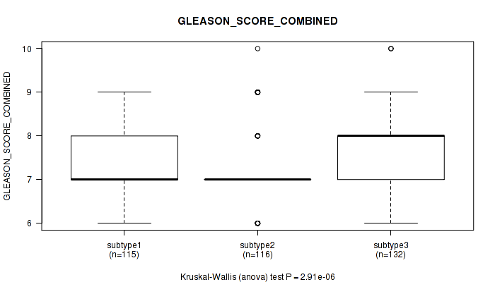
'MIRSEQ CNMF' versus 'GLEASON_SCORE_PRIMARY'

P value = 6.44e-06 (Kruskal-Wallis (anova)), Q value = 0.00086

Table S100. Clustering Approach #7: 'MIRSEQ CNMF' versus Clinical Feature #9: 'GLEASON_SCORE_PRIMARY'

	nPatients	Mean (Std.Dev)
ALL	363	3.6 (0.6)
subtype1	115	3.5 (0.6)
subtype2	116	3.5 (0.6)
subtype3	132	3.8 (0.6)

Figure S93. Get High-res Image Clustering Approach #7: 'MIRSEQ CNMF' versus Clinical Feature #9: 'GLEASON_SCORE_PRIMARY'

'MIRSEQ CNMF' versus 'GLEASON_SCORE_SECONDARY'

P value = 0.0237 (Kruskal-Wallis (anova)), Q value = 1

Table S101. Clustering Approach #7: 'MIRSEQ CNMF' versus Clinical Feature #10: 'GLEASON_SCORE_SECONDARY'

	nPatients	Mean (Std.Dev)
ALL	363	3.9 (0.6)
subtype1	115	3.9 (0.6)
subtype2	116	3.7 (0.6)
subtype3	132	3.9 (0.7)

Figure S94. Get High-res Image Clustering Approach #7: 'MIRSEQ CNMF' versus Clinical Feature #10: 'GLEASON_SCORE_SECONDARY'

'MIRSEQ CNMF' versus 'GLEASON_SCORE'

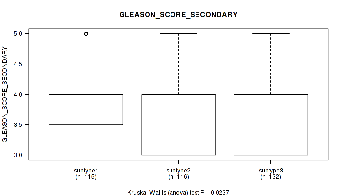
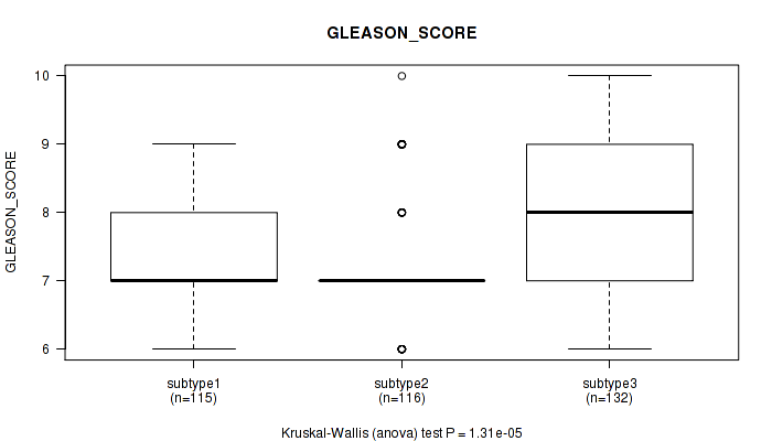
P value = 1.31e-05 (Kruskal-Wallis (anova)), Q value = 0.0017

Table S102. Clustering Approach #7: 'MIRSEQ CNMF' versus Clinical Feature #11: 'GLEASON_SCORE'

	nPatients	Mean (Std.Dev)
ALL	363	7.5 (0.9)
subtype1	115	7.5 (0.9)
subtype2	116	7.3 (0.9)
subtype3	132	7.8 (0.9)

Figure S95. Get High-res Image Clustering Approach #7: 'MIRSEQ CNMF' versus Clinical Feature #11: 'GLEASON_SCORE'

'MIRSEQ CNMF' versus 'PSA_RESULT_PREOP'

P value = 0.0607 (Kruskal-Wallis (anova)), Q value = 1

Table S103. Clustering Approach #7: 'MIRSEQ CNMF' versus Clinical Feature #12: 'PSA_RESULT_PREOP'

	nPatients	Mean (Std.Dev)
ALL	361	10.6 (11.4)
subtype1	114	10.1 (13.5)
subtype2	115	9.7 (9.6)
subtype3	132	11.9 (10.9)

Figure S96. Get High-res Image Clustering Approach #7: 'MIRSEQ CNMF' versus Clinical Feature #12: 'PSA_RESULT_PREOP'

'MIRSEQ CNMF' versus 'PSA_VALUE'

P value = 0.0163 (Kruskal-Wallis (anova)), Q value = 1

Table S104. Clustering Approach #7: 'MIRSEQ CNMF' versus Clinical Feature #13: 'PSA_VALUE'

	nPatients	Mean (Std.Dev)
ALL	314	1.0 (3.5)
subtype1	104	1.3 (4.6)
subtype2	98	0.1 (0.3)
subtype3	112	1.4 (3.7)

Figure S97. Get High-res Image Clustering Approach #7: 'MIRSEQ CNMF' versus Clinical Feature #13: 'PSA_VALUE'

'MIRSEQ CNMF' versus 'RACE'

P value = 0.218 (Fisher's exact test), Q value = 1

Table S105. Clustering Approach #7: 'MIRSEQ CNMF' versus Clinical Feature #14: 'RACE'

nPatients	ASIAN	BLACK OR AFRICAN AMERICAN	WHITE
ALL	2	7	146
subtype1	1	0	39
subtype2	1	3	69
subtype3	0	4	38

Figure S98. Get High-res Image Clustering Approach #7: 'MIRSEQ CNMF' versus Clinical Feature #14: 'RACE'

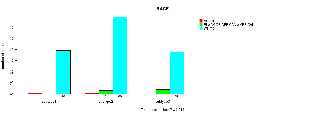
Clustering Approach #8: 'MIRSEQ CHIERARCHICAL'

Table S106. Description of clustering approach #8: 'MIRSEQ CHIERARCHICAL'

Cluster Labels	1	2	3	4	5
Number of samples	112	72	46	80	53

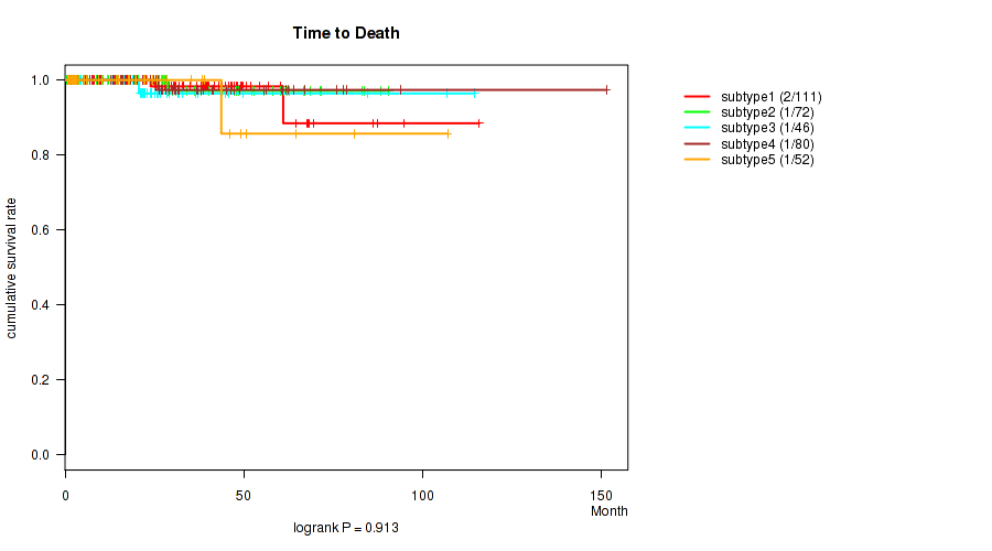
'MIRSEQ CHIERARCHICAL' versus 'Time to Death'

P value = 0.913 (logrank test), Q value = 1

Table S107. Clustering Approach #8: 'MIRSEQ CHIERARCHICAL' versus Clinical Feature #1: 'Time to Death'

	nPatients	nDeath	Duration Range (Median), Month
ALL	361	6	0.3 - 151.4 (23.9)
subtype1	111	2	1.0 - 115.9 (27.2)
subtype2	72	1	0.3 - 90.5 (28.0)
subtype3	46	1	1.0 - 114.6 (22.2)
subtype4	80	1	0.8 - 151.4 (25.2)
subtype5	52	1	0.7 - 107.0 (14.8)

Figure S99. Get High-res Image Clustering Approach #8: 'MIRSEQ CHIERARCHICAL' versus Clinical Feature #1: 'Time to Death'

'MIRSEQ CHIERARCHICAL' versus 'AGE'

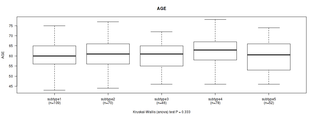
P value = 0.333 (Kruskal-Wallis (anova)), Q value = 1

Table S108. Clustering Approach #8: 'MIRSEQ CHIERARCHICAL' versus Clinical Feature #2: 'AGE'

	nPatients	Mean (Std.Dev)
ALL	355	60.8 (7.0)
subtype1	109	60.3 (6.8)
subtype2	70	60.6 (7.0)
subtype3	46	60.3 (6.2)
subtype4	78	62.4 (7.1)
subtype5	52	60.4 (7.6)

Figure S100. Get High-res Image Clustering Approach #8: 'MIRSEQ CHIERARCHICAL' versus Clinical Feature #2: 'AGE'

'MIRSEQ CHIERARCHICAL' versus 'PATHOLOGY.T.STAGE'

P value = 3e-05 (Fisher's exact test), Q value = 0.0037

Table S109. Clustering Approach #8: 'MIRSEQ CHIERARCHICAL' versus Clinical Feature #3: 'PATHOLOGY.T.STAGE'

nPatients	T2	T3	T4
ALL	149	208	4
subtype1	47	63	0
subtype2	37	31	4
subtype3	17	29	0
subtype4	18	62	0
subtype5	30	23	0

Figure S101. Get High-res Image Clustering Approach #8: 'MIRSEQ CHIERARCHICAL' versus Clinical Feature #3: 'PATHOLOGY.T.STAGE'

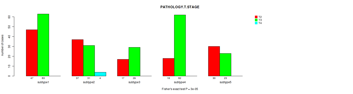
'MIRSEQ CHIERARCHICAL' versus 'PATHOLOGY.N.STAGE'

P value = 0.00091 (Fisher's exact test), Q value = 0.1

Table S110. Clustering Approach #8: 'MIRSEQ CHIERARCHICAL' versus Clinical Feature #4: 'PATHOLOGY.N.STAGE'

nPatients	0	1
ALL	263	44
subtype1	82	13
subtype2	55	2
subtype3	33	7
subtype4	54	20
subtype5	39	2

Figure S102. Get High-res Image Clustering Approach #8: 'MIRSEQ CHIERARCHICAL' versus Clinical Feature #4: 'PATHOLOGY.N.STAGE'

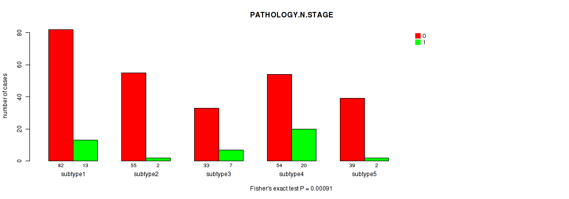
'MIRSEQ CHIERARCHICAL' versus 'HISTOLOGICAL.TYPE'

P value = 0.49 (Fisher's exact test), Q value = 1

Table S111. Clustering Approach #8: 'MIRSEQ CHIERARCHICAL' versus Clinical Feature #5: 'HISTOLOGICAL.TYPE'

nPatients	PROSTATE ADENOCARCINOMA OTHER SUBTYPE	PROSTATE ADENOCARCINOMA ACINAR TYPE
ALL	14	349
subtype1	6	106
subtype2	1	71
subtype3	1	45
subtype4	5	75
subtype5	1	52

Figure S103. Get High-res Image Clustering Approach #8: 'MIRSEQ CHIERARCHICAL' versus Clinical Feature #5: 'HISTOLOGICAL.TYPE'

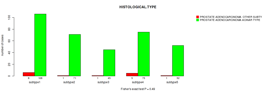
'MIRSEQ CHIERARCHICAL' versus 'COMPLETENESS.OF.RESECTION'

P value = 0.0486 (Fisher's exact test), Q value = 1

Table S112. Clustering Approach #8: 'MIRSEQ CHIERARCHICAL' versus Clinical Feature #6: 'COMPLETENESS.OF.RESECTION'

nPatients	R0	R1	R2	RX
ALL	242	91	5	11
subtype1	82	24	0	4
subtype2	46	21	1	2
subtype3	32	10	0	2
subtype4	44	30	2	2
subtype5	38	6	2	1

Figure S104. Get High-res Image Clustering Approach #8: 'MIRSEQ CHIERARCHICAL' versus Clinical Feature #6: 'COMPLETENESS.OF.RESECTION'

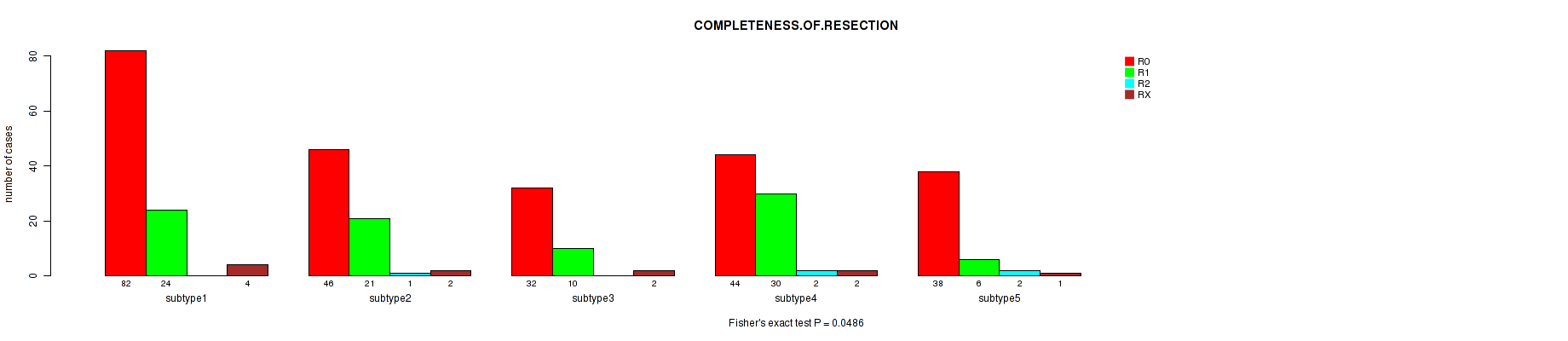
'MIRSEQ CHIERARCHICAL' versus 'NUMBER.OF.LYMPH.NODES'

P value = 0.000816 (Kruskal-Wallis (anova)), Q value = 0.091

Table S113. Clustering Approach #8: 'MIRSEQ CHIERARCHICAL' versus Clinical Feature #7: 'NUMBER.OF.LYMPH.NODES'

	nPatients	Mean (Std.Dev)
ALL	303	0.3 (1.3)
subtype1	92	0.3 (0.8)
subtype2	56	0.0 (0.2)
subtype3	40	0.2 (0.6)
subtype4	74	0.9 (2.4)
subtype5	41	0.1 (0.3)

Figure S105. Get High-res Image Clustering Approach #8: 'MIRSEQ CHIERARCHICAL' versus Clinical Feature #7: 'NUMBER.OF.LYMPH.NODES'

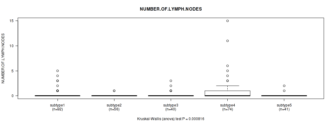
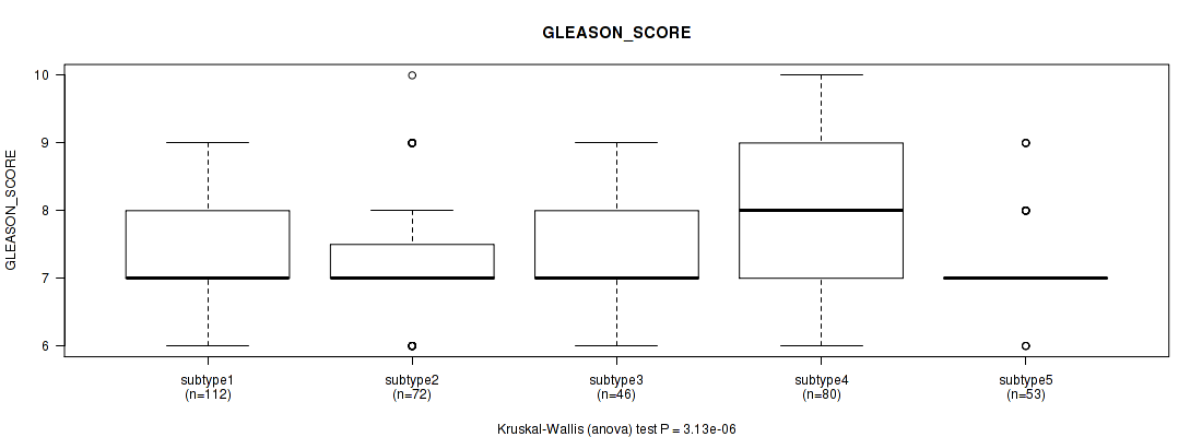
'MIRSEQ CHIERARCHICAL' versus 'GLEASON_SCORE_COMBINED'

P value = 6.91e-08 (Kruskal-Wallis (anova)), Q value = 9.5e-06

Table S114. Clustering Approach #8: 'MIRSEQ CHIERARCHICAL' versus Clinical Feature #8: 'GLEASON_SCORE_COMBINED'

	nPatients	Mean (Std.Dev)
ALL	363	7.4 (0.9)
subtype1	112	7.4 (0.9)
subtype2	72	7.2 (0.9)
subtype3	46	7.5 (0.9)
subtype4	80	8.0 (0.9)
subtype5	53	7.2 (0.7)

Figure S106. Get High-res Image Clustering Approach #8: 'MIRSEQ CHIERARCHICAL' versus Clinical Feature #8: 'GLEASON_SCORE_COMBINED'

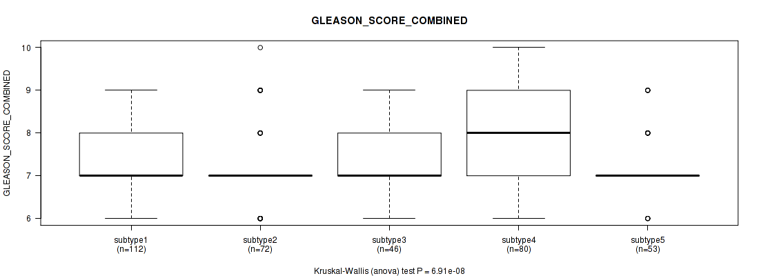
'MIRSEQ CHIERARCHICAL' versus 'GLEASON_SCORE_PRIMARY'

P value = 2.31e-05 (Kruskal-Wallis (anova)), Q value = 0.003

Table S115. Clustering Approach #8: 'MIRSEQ CHIERARCHICAL' versus Clinical Feature #9: 'GLEASON_SCORE_PRIMARY'

	nPatients	Mean (Std.Dev)
ALL	363	3.6 (0.6)
subtype1	112	3.5 (0.6)
subtype2	72	3.5 (0.6)
subtype3	46	3.6 (0.6)
subtype4	80	3.9 (0.6)
subtype5	53	3.5 (0.5)

Figure S107. Get High-res Image Clustering Approach #8: 'MIRSEQ CHIERARCHICAL' versus Clinical Feature #9: 'GLEASON_SCORE_PRIMARY'

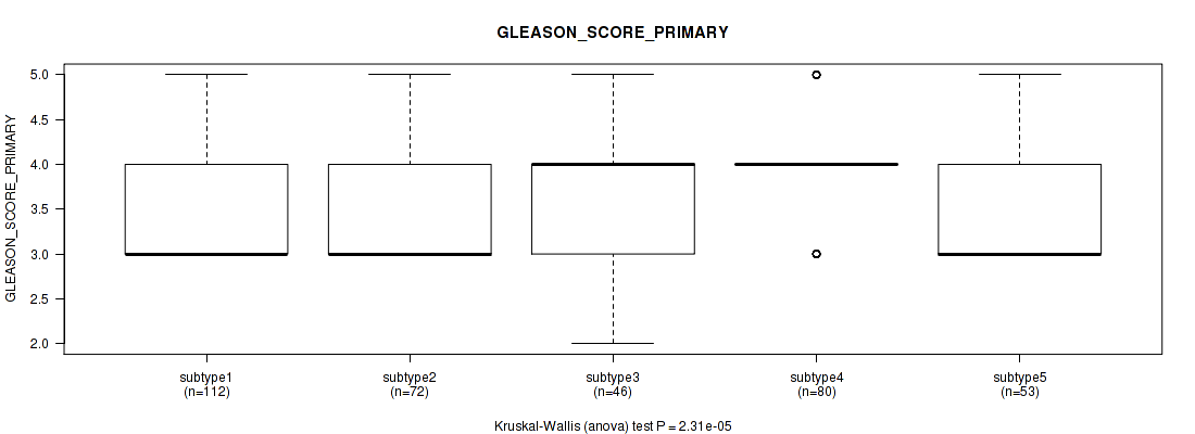
'MIRSEQ CHIERARCHICAL' versus 'GLEASON_SCORE_SECONDARY'

P value = 0.0112 (Kruskal-Wallis (anova)), Q value = 0.98

Table S116. Clustering Approach #8: 'MIRSEQ CHIERARCHICAL' versus Clinical Feature #10: 'GLEASON_SCORE_SECONDARY'

	nPatients	Mean (Std.Dev)
ALL	363	3.9 (0.6)
subtype1	112	3.9 (0.6)
subtype2	72	3.7 (0.6)
subtype3	46	3.9 (0.7)
subtype4	80	4.0 (0.7)
subtype5	53	3.7 (0.6)

Figure S108. Get High-res Image Clustering Approach #8: 'MIRSEQ CHIERARCHICAL' versus Clinical Feature #10: 'GLEASON_SCORE_SECONDARY'

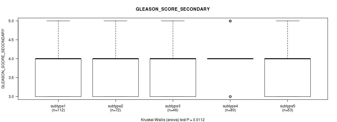
'MIRSEQ CHIERARCHICAL' versus 'GLEASON_SCORE'

P value = 3.13e-06 (Kruskal-Wallis (anova)), Q value = 0.00042

Table S117. Clustering Approach #8: 'MIRSEQ CHIERARCHICAL' versus Clinical Feature #11: 'GLEASON_SCORE'

	nPatients	Mean (Std.Dev)
ALL	363	7.5 (0.9)
subtype1	112	7.4 (0.9)
subtype2	72	7.3 (1.0)
subtype3	46	7.5 (0.9)
subtype4	80	8.0 (1.0)
subtype5	53	7.3 (0.7)

Figure S109. Get High-res Image Clustering Approach #8: 'MIRSEQ CHIERARCHICAL' versus Clinical Feature #11: 'GLEASON_SCORE'

'MIRSEQ CHIERARCHICAL' versus 'PSA_RESULT_PREOP'

P value = 0.321 (Kruskal-Wallis (anova)), Q value = 1

Table S118. Clustering Approach #8: 'MIRSEQ CHIERARCHICAL' versus Clinical Feature #12: 'PSA_RESULT_PREOP'

	nPatients	Mean (Std.Dev)
ALL	361	10.6 (11.4)
subtype1	110	10.6 (13.9)
subtype2	72	11.0 (11.7)
subtype3	46	9.6 (7.4)
subtype4	80	12.3 (12.0)
subtype5	53	8.3 (5.8)

Figure S110. Get High-res Image Clustering Approach #8: 'MIRSEQ CHIERARCHICAL' versus Clinical Feature #12: 'PSA_RESULT_PREOP'

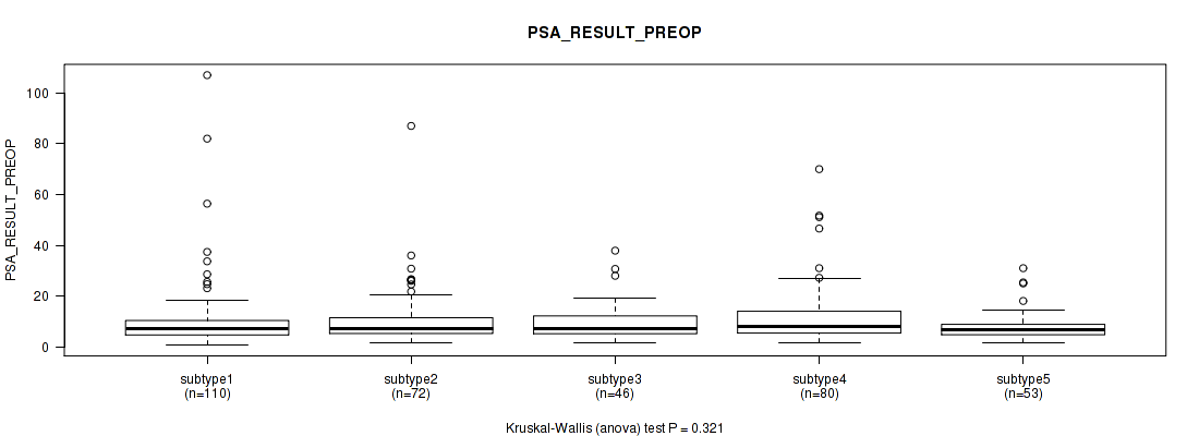
'MIRSEQ CHIERARCHICAL' versus 'PSA_VALUE'

P value = 0.379 (Kruskal-Wallis (anova)), Q value = 1

Table S119. Clustering Approach #8: 'MIRSEQ CHIERARCHICAL' versus Clinical Feature #13: 'PSA_VALUE'

	nPatients	Mean (Std.Dev)
ALL	314	1.0 (3.5)
subtype1	102	1.2 (4.5)
subtype2	67	0.2 (0.3)
subtype3	41	0.8 (2.4)
subtype4	62	1.6 (4.3)
subtype5	42	1.1 (3.0)

Figure S111. Get High-res Image Clustering Approach #8: 'MIRSEQ CHIERARCHICAL' versus Clinical Feature #13: 'PSA_VALUE'

'MIRSEQ CHIERARCHICAL' versus 'RACE'

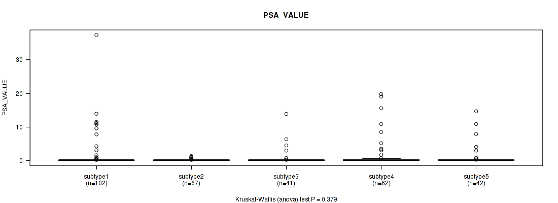
P value = 0.706 (Fisher's exact test), Q value = 1

Table S120. Clustering Approach #8: 'MIRSEQ CHIERARCHICAL' versus Clinical Feature #14: 'RACE'

nPatients	ASIAN	BLACK OR AFRICAN AMERICAN	WHITE
ALL	2	7	146
subtype1	1	1	51
subtype2	0	3	30
subtype3	0	0	18
subtype4	0	0	9
subtype5	1	3	38

Figure S112. Get High-res Image Clustering Approach #8: 'MIRSEQ CHIERARCHICAL' versus Clinical Feature #14: 'RACE'

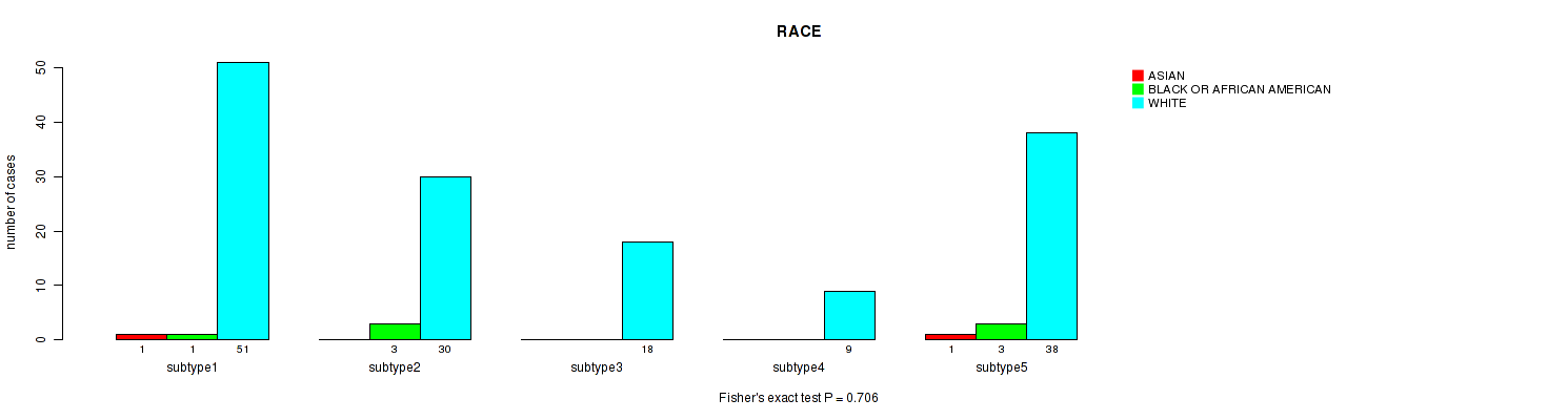
Clustering Approach #9: 'MIRseq Mature CNMF subtypes'

Table S121. Description of clustering approach #9: 'MIRseq Mature CNMF subtypes'

Cluster Labels	1	2	3	4
Number of samples	50	61	33	80

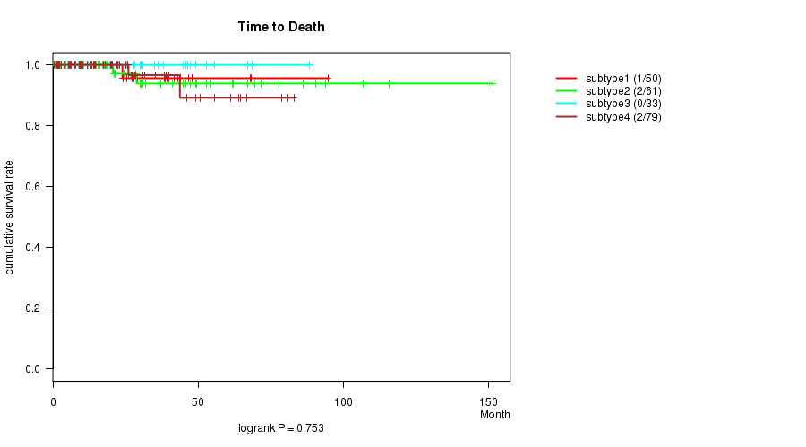
'MIRseq Mature CNMF subtypes' versus 'Time to Death'

P value = 0.753 (logrank test), Q value = 1

Table S122. Clustering Approach #9: 'MIRseq Mature CNMF subtypes' versus Clinical Feature #1: 'Time to Death'

	nPatients	nDeath	Duration Range (Median), Month
ALL	223	5	0.3 - 151.4 (22.3)
subtype1	50	1	1.0 - 94.7 (22.0)
subtype2	61	2	0.8 - 151.4 (28.5)
subtype3	33	0	1.1 - 88.2 (28.2)
subtype4	79	2	0.3 - 82.9 (19.9)

Figure S113. Get High-res Image Clustering Approach #9: 'MIRseq Mature CNMF subtypes' versus Clinical Feature #1: 'Time to Death'

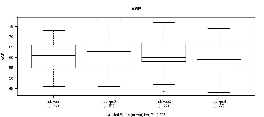
'MIRseq Mature CNMF subtypes' versus 'AGE'

P value = 0.235 (Kruskal-Wallis (anova)), Q value = 1

Table S123. Clustering Approach #9: 'MIRseq Mature CNMF subtypes' versus Clinical Feature #2: 'AGE'

	nPatients	Mean (Std.Dev)
ALL	218	60.5 (7.1)
subtype1	47	60.3 (7.2)
subtype2	61	61.9 (6.4)
subtype3	33	60.9 (7.4)
subtype4	77	59.2 (7.4)

Figure S114. Get High-res Image Clustering Approach #9: 'MIRseq Mature CNMF subtypes' versus Clinical Feature #2: 'AGE'

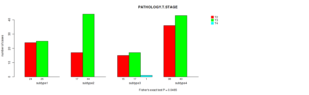
'MIRseq Mature CNMF subtypes' versus 'PATHOLOGY.T.STAGE'

P value = 0.0465 (Fisher's exact test), Q value = 1

Table S124. Clustering Approach #9: 'MIRseq Mature CNMF subtypes' versus Clinical Feature #3: 'PATHOLOGY.T.STAGE'

nPatients	T2	T3	T4
ALL	92	129	1
subtype1	24	25	0
subtype2	17	44	0
subtype3	15	17	1
subtype4	36	43	0

Figure S115. Get High-res Image Clustering Approach #9: 'MIRseq Mature CNMF subtypes' versus Clinical Feature #3: 'PATHOLOGY.T.STAGE'

'MIRseq Mature CNMF subtypes' versus 'PATHOLOGY.N.STAGE'

P value = 0.392 (Fisher's exact test), Q value = 1

Table S125. Clustering Approach #9: 'MIRseq Mature CNMF subtypes' versus Clinical Feature #4: 'PATHOLOGY.N.STAGE'

nPatients	0	1
ALL	164	26
subtype1	34	7
subtype2	49	6
subtype3	21	6
subtype4	60	7

Figure S116. Get High-res Image Clustering Approach #9: 'MIRseq Mature CNMF subtypes' versus Clinical Feature #4: 'PATHOLOGY.N.STAGE'

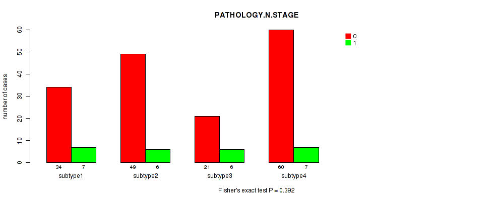
'MIRseq Mature CNMF subtypes' versus 'HISTOLOGICAL.TYPE'

P value = 0.0582 (Fisher's exact test), Q value = 1

Table S126. Clustering Approach #9: 'MIRseq Mature CNMF subtypes' versus Clinical Feature #5: 'HISTOLOGICAL.TYPE'

nPatients	PROSTATE ADENOCARCINOMA OTHER SUBTYPE	PROSTATE ADENOCARCINOMA ACINAR TYPE
ALL	8	216
subtype1	3	47
subtype2	4	57
subtype3	1	32
subtype4	0	80

Figure S117. Get High-res Image Clustering Approach #9: 'MIRseq Mature CNMF subtypes' versus Clinical Feature #5: 'HISTOLOGICAL.TYPE'

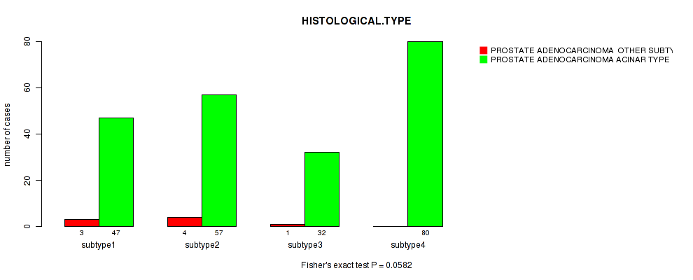
'MIRseq Mature CNMF subtypes' versus 'COMPLETENESS.OF.RESECTION'

P value = 0.0392 (Fisher's exact test), Q value = 1

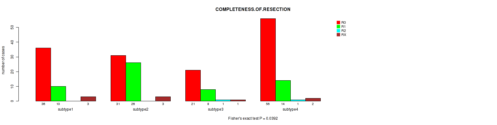
Table S127. Clustering Approach #9: 'MIRseq Mature CNMF subtypes' versus Clinical Feature #6: 'COMPLETENESS.OF.RESECTION'

nPatients	R0	R1	R2	RX
ALL	144	58	2	9
subtype1	36	10	0	3
subtype2	31	26	0	3
subtype3	21	8	1	1
subtype4	56	14	1	2

Figure S118. Get High-res Image Clustering Approach #9: 'MIRseq Mature CNMF subtypes' versus Clinical Feature #6: 'COMPLETENESS.OF.RESECTION'

'MIRseq Mature CNMF subtypes' versus 'NUMBER.OF.LYMPH.NODES'

P value = 0.399 (Kruskal-Wallis (anova)), Q value = 1

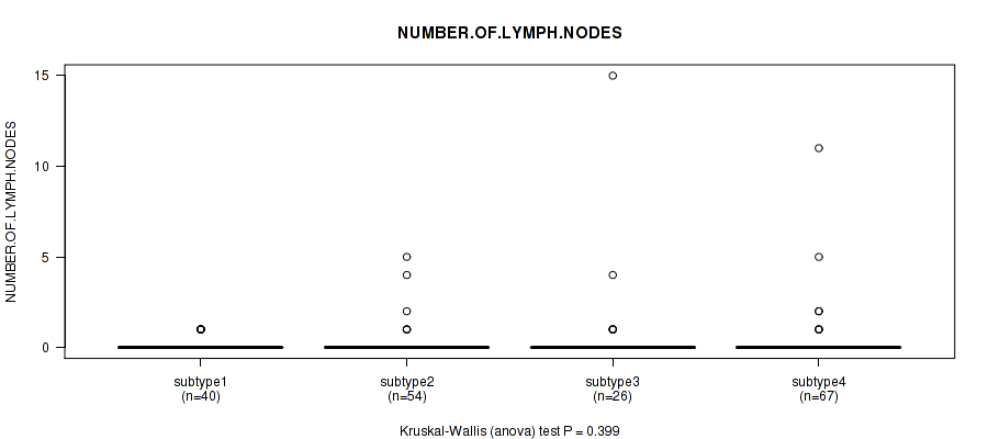
Table S128. Clustering Approach #9: 'MIRseq Mature CNMF subtypes' versus Clinical Feature #7: 'NUMBER.OF.LYMPH.NODES'

	nPatients	Mean (Std.Dev)
ALL	187	0.4 (1.5)
subtype1	40	0.2 (0.4)
subtype2	54	0.3 (0.9)
subtype3	26	0.9 (3.0)
subtype4	67	0.3 (1.5)

Figure S119. Get High-res Image Clustering Approach #9: 'MIRseq Mature CNMF subtypes' versus Clinical Feature #7: 'NUMBER.OF.LYMPH.NODES'

'MIRseq Mature CNMF subtypes' versus 'GLEASON_SCORE_COMBINED'

P value = 0.0012 (Kruskal-Wallis (anova)), Q value = 0.13

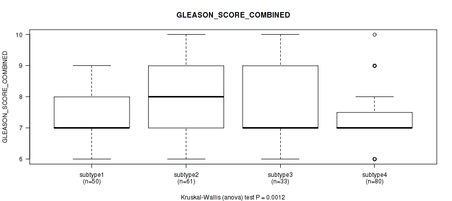
Table S129. Clustering Approach #9: 'MIRseq Mature CNMF subtypes' versus Clinical Feature #8: 'GLEASON_SCORE_COMBINED'

	nPatients	Mean (Std.Dev)
ALL	224	7.5 (1.0)
subtype1	50	7.3 (0.9)
subtype2	61	7.9 (1.0)
subtype3	33	7.5 (1.2)
subtype4	80	7.3 (0.8)

Figure S120. Get High-res Image Clustering Approach #9: 'MIRseq Mature CNMF subtypes' versus Clinical Feature #8: 'GLEASON_SCORE_COMBINED'

'MIRseq Mature CNMF subtypes' versus 'GLEASON_SCORE_PRIMARY'

P value = 0.00105 (Kruskal-Wallis (anova)), Q value = 0.11

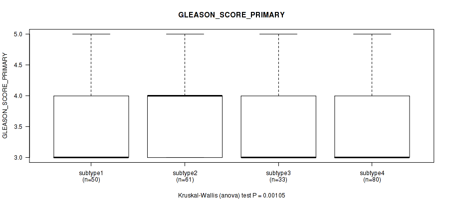
Table S130. Clustering Approach #9: 'MIRseq Mature CNMF subtypes' versus Clinical Feature #9: 'GLEASON_SCORE_PRIMARY'

	nPatients	Mean (Std.Dev)
ALL	224	3.6 (0.6)
subtype1	50	3.4 (0.5)
subtype2	61	3.8 (0.6)
subtype3	33	3.5 (0.7)
subtype4	80	3.5 (0.6)

Figure S121. Get High-res Image Clustering Approach #9: 'MIRseq Mature CNMF subtypes' versus Clinical Feature #9: 'GLEASON_SCORE_PRIMARY'

'MIRseq Mature CNMF subtypes' versus 'GLEASON_SCORE_SECONDARY'

P value = 0.0799 (Kruskal-Wallis (anova)), Q value = 1

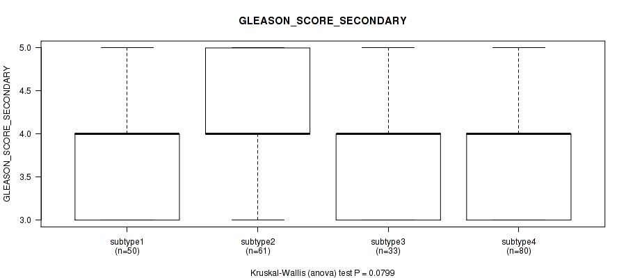
Table S131. Clustering Approach #9: 'MIRseq Mature CNMF subtypes' versus Clinical Feature #10: 'GLEASON_SCORE_SECONDARY'

	nPatients	Mean (Std.Dev)
ALL	224	3.9 (0.7)
subtype1	50	3.9 (0.7)
subtype2	61	4.1 (0.7)
subtype3	33	3.9 (0.7)
subtype4	80	3.8 (0.6)

Figure S122. Get High-res Image Clustering Approach #9: 'MIRseq Mature CNMF subtypes' versus Clinical Feature #10: 'GLEASON_SCORE_SECONDARY'

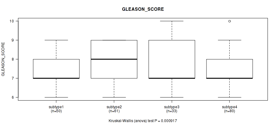
'MIRseq Mature CNMF subtypes' versus 'GLEASON_SCORE'

P value = 0.000917 (Kruskal-Wallis (anova)), Q value = 0.1

Table S132. Clustering Approach #9: 'MIRseq Mature CNMF subtypes' versus Clinical Feature #11: 'GLEASON_SCORE'

	nPatients	Mean (Std.Dev)
ALL	224	7.5 (1.0)
subtype1	50	7.3 (1.0)
subtype2	61	7.9 (1.0)
subtype3	33	7.7 (1.2)
subtype4	80	7.3 (0.8)

Figure S123. Get High-res Image Clustering Approach #9: 'MIRseq Mature CNMF subtypes' versus Clinical Feature #11: 'GLEASON_SCORE'

'MIRseq Mature CNMF subtypes' versus 'PSA_RESULT_PREOP'

P value = 0.432 (Kruskal-Wallis (anova)), Q value = 1

Table S133. Clustering Approach #9: 'MIRseq Mature CNMF subtypes' versus Clinical Feature #12: 'PSA_RESULT_PREOP'

	nPatients	Mean (Std.Dev)
ALL	224	9.7 (9.5)
subtype1	50	10.9 (11.8)
subtype2	61	10.3 (11.0)
subtype3	33	9.1 (8.9)
subtype4	80	8.7 (6.4)

Figure S124. Get High-res Image Clustering Approach #9: 'MIRseq Mature CNMF subtypes' versus Clinical Feature #12: 'PSA_RESULT_PREOP'

'MIRseq Mature CNMF subtypes' versus 'PSA_VALUE'

P value = 0.252 (Kruskal-Wallis (anova)), Q value = 1

Table S134. Clustering Approach #9: 'MIRseq Mature CNMF subtypes' versus Clinical Feature #13: 'PSA_VALUE'

	nPatients	Mean (Std.Dev)
ALL	193	0.7 (2.4)
subtype1	47	1.4 (3.9)
subtype2	51	0.2 (0.5)
subtype3	29	0.5 (2.1)
subtype4	66	0.6 (1.8)

Figure S125. Get High-res Image Clustering Approach #9: 'MIRseq Mature CNMF subtypes' versus Clinical Feature #13: 'PSA_VALUE'

'MIRseq Mature CNMF subtypes' versus 'RACE'

P value = 0.806 (Fisher's exact test), Q value = 1

Table S135. Clustering Approach #9: 'MIRseq Mature CNMF subtypes' versus Clinical Feature #14: 'RACE'

nPatients	ASIAN	BLACK OR AFRICAN AMERICAN	WHITE
ALL	1	3	91
subtype1	0	0	27
subtype2	0	0	3
subtype3	0	0	7
subtype4	1	3	54

Figure S126. Get High-res Image Clustering Approach #9: 'MIRseq Mature CNMF subtypes' versus Clinical Feature #14: 'RACE'

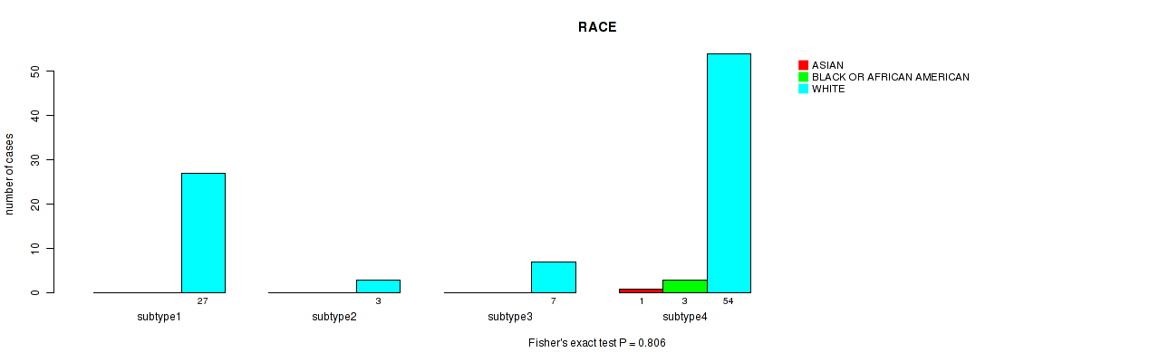
Clustering Approach #10: 'MIRseq Mature cHierClus subtypes'

Table S136. Description of clustering approach #10: 'MIRseq Mature cHierClus subtypes'

Cluster Labels	1	2	3	4	5	6
Number of samples	46	26	17	52	25	58

'MIRseq Mature cHierClus subtypes' versus 'Time to Death'

P value = 0.847 (logrank test), Q value = 1

Table S137. Clustering Approach #10: 'MIRseq Mature cHierClus subtypes' versus Clinical Feature #1: 'Time to Death'

	nPatients	nDeath	Duration Range (Median), Month
ALL	223	5	0.3 - 151.4 (22.3)
subtype1	46	1	1.2 - 94.7 (22.0)
subtype2	26	1	0.3 - 88.2 (24.2)
subtype3	17	1	1.1 - 107.0 (25.5)
subtype4	52	1	0.8 - 151.4 (26.3)
subtype5	25	0	1.0 - 68.3 (28.9)
subtype6	57	1	1.1 - 82.9 (19.6)

Figure S127. Get High-res Image Clustering Approach #10: 'MIRseq Mature cHierClus subtypes' versus Clinical Feature #1: 'Time to Death'

'MIRseq Mature cHierClus subtypes' versus 'AGE'

P value = 0.363 (Kruskal-Wallis (anova)), Q value = 1

Table S138. Clustering Approach #10: 'MIRseq Mature cHierClus subtypes' versus Clinical Feature #2: 'AGE'

	nPatients	Mean (Std.Dev)
ALL	218	60.5 (7.1)
subtype1	43	59.3 (6.6)
subtype2	25	59.2 (8.3)
subtype3	17	61.2 (6.5)
subtype4	52	62.4 (6.9)
subtype5	25	60.3 (7.6)
subtype6	56	60.0 (7.2)

Figure S128. Get High-res Image Clustering Approach #10: 'MIRseq Mature cHierClus subtypes' versus Clinical Feature #2: 'AGE'

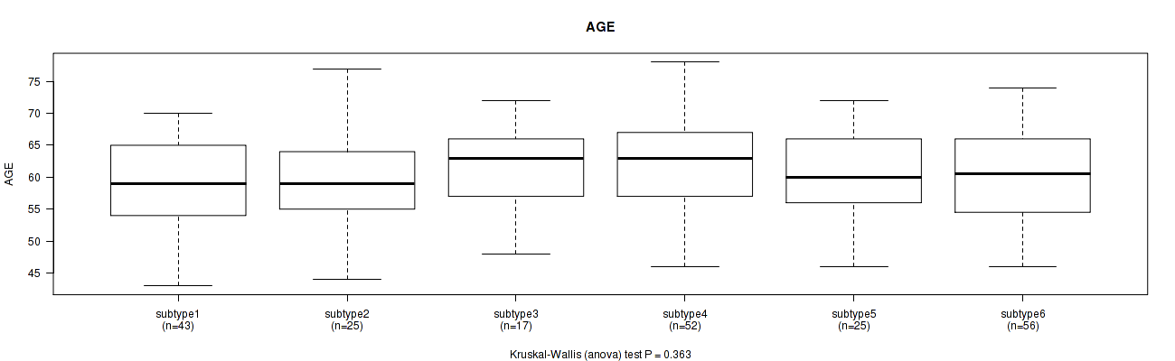
'MIRseq Mature cHierClus subtypes' versus 'PATHOLOGY.T.STAGE'

P value = 0.00209 (Fisher's exact test), Q value = 0.22

Table S139. Clustering Approach #10: 'MIRseq Mature cHierClus subtypes' versus Clinical Feature #3: 'PATHOLOGY.T.STAGE'

nPatients	T2	T3	T4
ALL	92	129	1
subtype1	24	21	0
subtype2	17	9	0
subtype3	3	14	0
subtype4	14	38	0
subtype5	8	15	1
subtype6	26	32	0

Figure S129. Get High-res Image Clustering Approach #10: 'MIRseq Mature cHierClus subtypes' versus Clinical Feature #3: 'PATHOLOGY.T.STAGE'

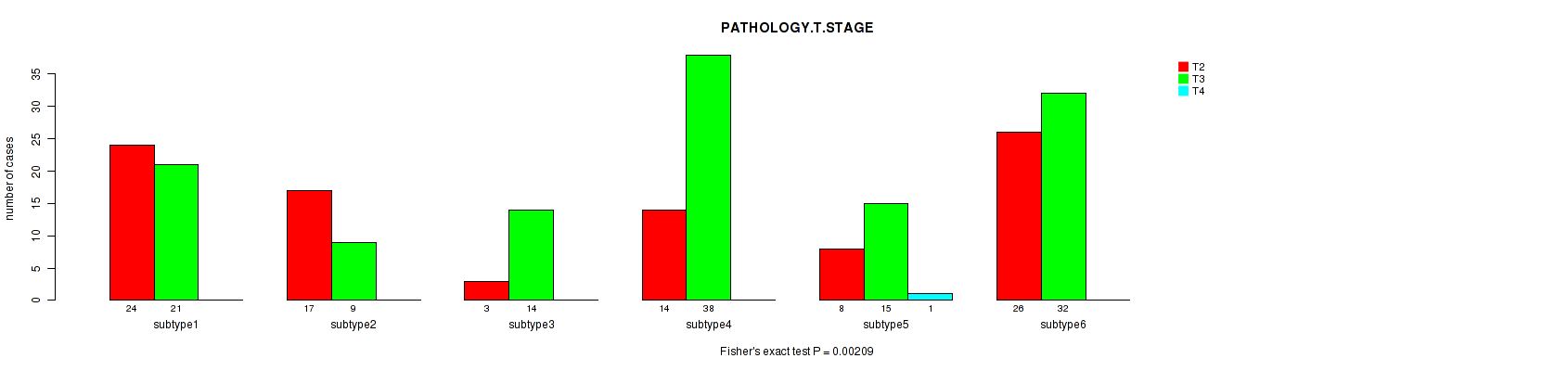
'MIRseq Mature cHierClus subtypes' versus 'PATHOLOGY.N.STAGE'

P value = 0.00051 (Fisher's exact test), Q value = 0.058

Table S140. Clustering Approach #10: 'MIRseq Mature cHierClus subtypes' versus Clinical Feature #4: 'PATHOLOGY.N.STAGE'

nPatients	0	1
ALL	164	26
subtype1	27	5
subtype2	20	0
subtype3	8	8
subtype4	43	5
subtype5	19	5
subtype6	47	3

Figure S130. Get High-res Image Clustering Approach #10: 'MIRseq Mature cHierClus subtypes' versus Clinical Feature #4: 'PATHOLOGY.N.STAGE'

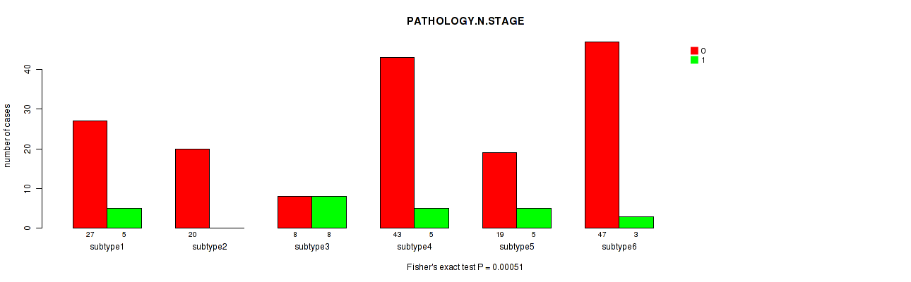
'MIRseq Mature cHierClus subtypes' versus 'HISTOLOGICAL.TYPE'

P value = 0.148 (Fisher's exact test), Q value = 1

Table S141. Clustering Approach #10: 'MIRseq Mature cHierClus subtypes' versus Clinical Feature #5: 'HISTOLOGICAL.TYPE'

nPatients	PROSTATE ADENOCARCINOMA OTHER SUBTYPE	PROSTATE ADENOCARCINOMA ACINAR TYPE
ALL	8	216
subtype1	4	42
subtype2	1	25
subtype3	1	16
subtype4	2	50
subtype5	0	25
subtype6	0	58

Figure S131. Get High-res Image Clustering Approach #10: 'MIRseq Mature cHierClus subtypes' versus Clinical Feature #5: 'HISTOLOGICAL.TYPE'

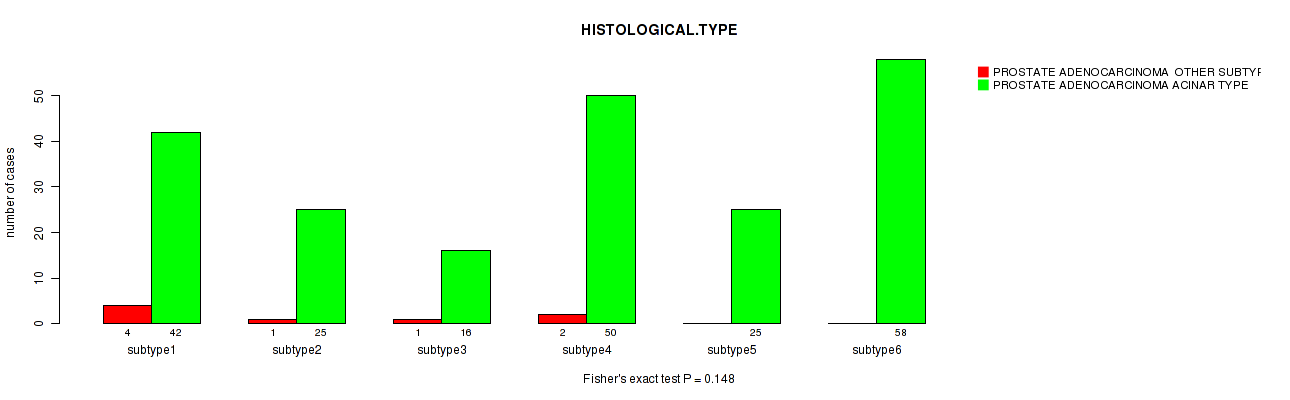
'MIRseq Mature cHierClus subtypes' versus 'COMPLETENESS.OF.RESECTION'

P value = 0.0355 (Fisher's exact test), Q value = 1

Table S142. Clustering Approach #10: 'MIRseq Mature cHierClus subtypes' versus Clinical Feature #6: 'COMPLETENESS.OF.RESECTION'

nPatients	R0	R1	R2	RX
ALL	144	58	2	9
subtype1	34	7	0	3
subtype2	20	4	1	0
subtype3	10	6	0	1
subtype4	25	24	0	2
subtype5	17	7	0	1
subtype6	38	10	1	2

Figure S132. Get High-res Image Clustering Approach #10: 'MIRseq Mature cHierClus subtypes' versus Clinical Feature #6: 'COMPLETENESS.OF.RESECTION'

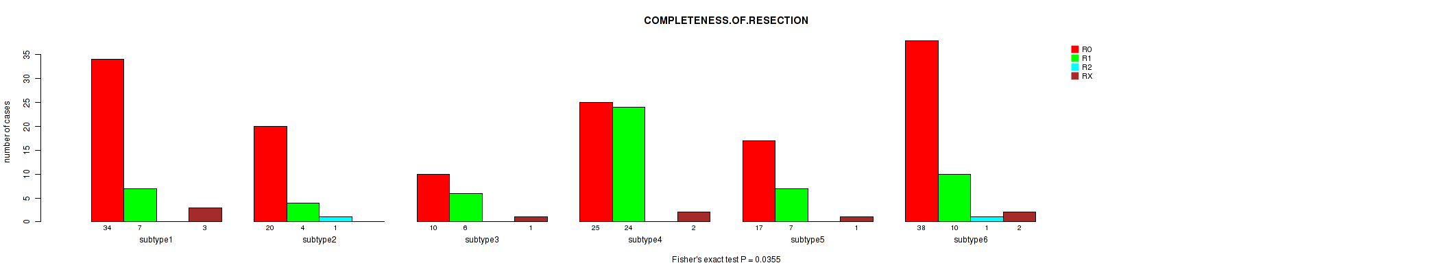
'MIRseq Mature cHierClus subtypes' versus 'NUMBER.OF.LYMPH.NODES'

P value = 9.93e-05 (Kruskal-Wallis (anova)), Q value = 0.012

Table S143. Clustering Approach #10: 'MIRseq Mature cHierClus subtypes' versus Clinical Feature #7: 'NUMBER.OF.LYMPH.NODES'

	nPatients	Mean (Std.Dev)
ALL	187	0.4 (1.5)
subtype1	29	0.3 (0.8)
subtype2	20	0.0 (0.0)
subtype3	16	2.3 (4.4)
subtype4	48	0.3 (1.0)
subtype5	24	0.2 (0.4)
subtype6	50	0.1 (0.3)

Figure S133. Get High-res Image Clustering Approach #10: 'MIRseq Mature cHierClus subtypes' versus Clinical Feature #7: 'NUMBER.OF.LYMPH.NODES'

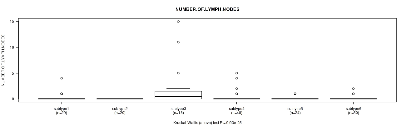
'MIRseq Mature cHierClus subtypes' versus 'GLEASON_SCORE_COMBINED'

P value = 0.000367 (Kruskal-Wallis (anova)), Q value = 0.043

Table S144. Clustering Approach #10: 'MIRseq Mature cHierClus subtypes' versus Clinical Feature #8: 'GLEASON_SCORE_COMBINED'

	nPatients	Mean (Std.Dev)
ALL	224	7.5 (1.0)
subtype1	46	7.4 (1.0)
subtype2	26	7.0 (1.0)
subtype3	17	8.0 (1.1)
subtype4	52	7.9 (1.1)
subtype5	25	7.3 (0.8)
subtype6	58	7.3 (0.8)

Figure S134. Get High-res Image Clustering Approach #10: 'MIRseq Mature cHierClus subtypes' versus Clinical Feature #8: 'GLEASON_SCORE_COMBINED'

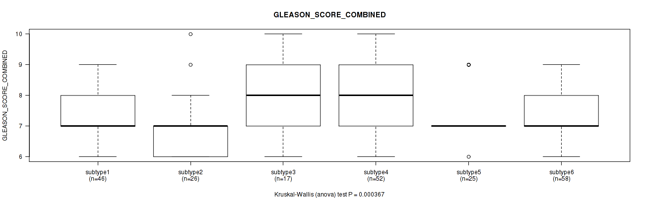
'MIRseq Mature cHierClus subtypes' versus 'GLEASON_SCORE_PRIMARY'

P value = 0.000278 (Kruskal-Wallis (anova)), Q value = 0.033

Table S145. Clustering Approach #10: 'MIRseq Mature cHierClus subtypes' versus Clinical Feature #9: 'GLEASON_SCORE_PRIMARY'

	nPatients	Mean (Std.Dev)
ALL	224	3.6 (0.6)
subtype1	46	3.6 (0.6)
subtype2	26	3.3 (0.5)
subtype3	17	4.0 (0.7)
subtype4	52	3.8 (0.6)
subtype5	25	3.4 (0.5)
subtype6	58	3.5 (0.5)

Figure S135. Get High-res Image Clustering Approach #10: 'MIRseq Mature cHierClus subtypes' versus Clinical Feature #9: 'GLEASON_SCORE_PRIMARY'

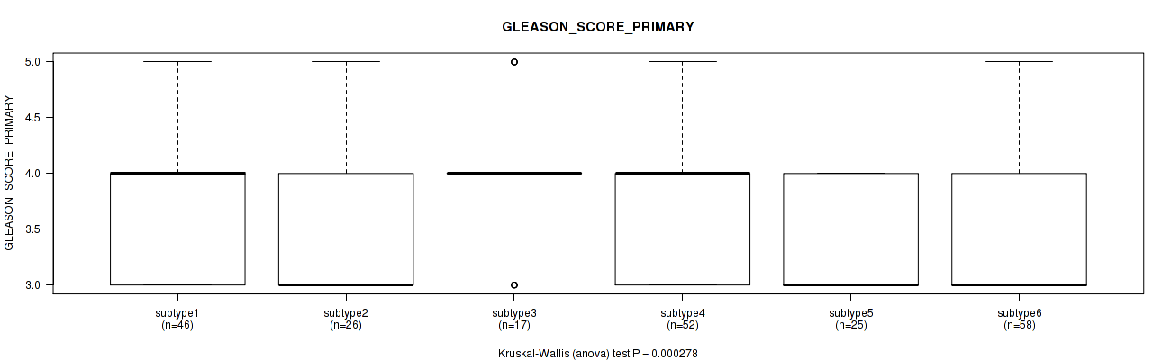
'MIRseq Mature cHierClus subtypes' versus 'GLEASON_SCORE_SECONDARY'

P value = 0.121 (Kruskal-Wallis (anova)), Q value = 1

Table S146. Clustering Approach #10: 'MIRseq Mature cHierClus subtypes' versus Clinical Feature #10: 'GLEASON_SCORE_SECONDARY'

	nPatients	Mean (Std.Dev)
ALL	224	3.9 (0.7)
subtype1	46	3.9 (0.7)
subtype2	26	3.7 (0.6)
subtype3	17	4.0 (0.6)
subtype4	52	4.1 (0.7)
subtype5	25	3.9 (0.6)
subtype6	58	3.8 (0.6)

Figure S136. Get High-res Image Clustering Approach #10: 'MIRseq Mature cHierClus subtypes' versus Clinical Feature #10: 'GLEASON_SCORE_SECONDARY'

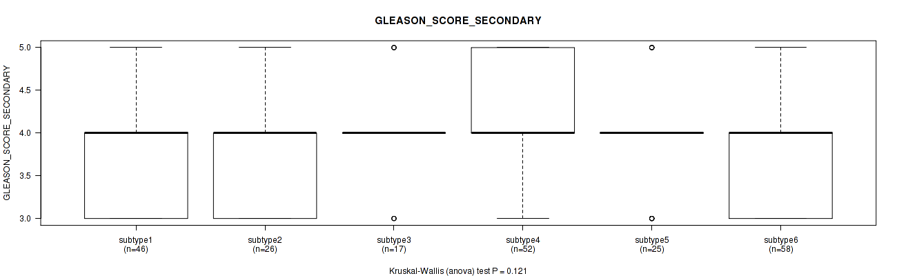
'MIRseq Mature cHierClus subtypes' versus 'GLEASON_SCORE'

P value = 0.000186 (Kruskal-Wallis (anova)), Q value = 0.022

Table S147. Clustering Approach #10: 'MIRseq Mature cHierClus subtypes' versus Clinical Feature #11: 'GLEASON_SCORE'

	nPatients	Mean (Std.Dev)
ALL	224	7.5 (1.0)
subtype1	46	7.5 (1.1)
subtype2	26	7.2 (1.0)
subtype3	17	8.2 (0.9)
subtype4	52	7.9 (1.0)
subtype5	25	7.2 (0.8)
subtype6	58	7.3 (0.8)

Figure S137. Get High-res Image Clustering Approach #10: 'MIRseq Mature cHierClus subtypes' versus Clinical Feature #11: 'GLEASON_SCORE'

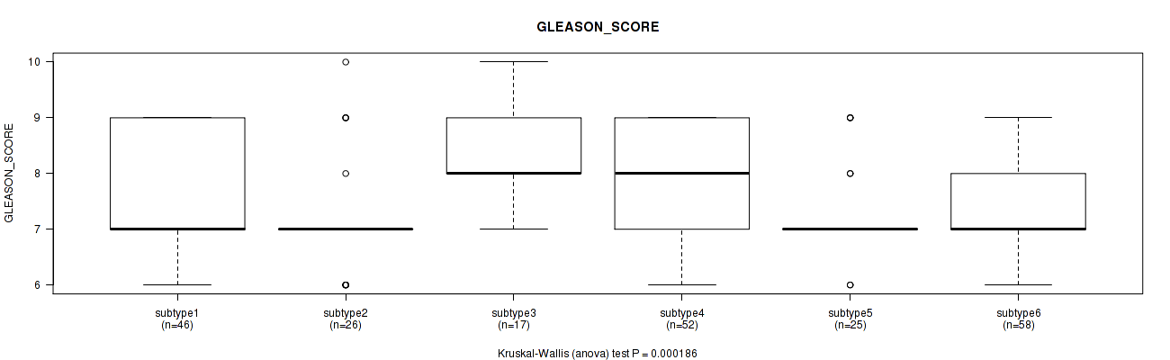
'MIRseq Mature cHierClus subtypes' versus 'PSA_RESULT_PREOP'

P value = 0.0701 (Kruskal-Wallis (anova)), Q value = 1

Table S148. Clustering Approach #10: 'MIRseq Mature cHierClus subtypes' versus Clinical Feature #12: 'PSA_RESULT_PREOP'

	nPatients	Mean (Std.Dev)
ALL	224	9.7 (9.5)
subtype1	46	7.3 (4.3)
subtype2	26	9.3 (6.7)
subtype3	17	11.4 (12.2)
subtype4	52	12.1 (15.4)
subtype5	25	11.8 (7.0)
subtype6	58	8.1 (5.3)

Figure S138. Get High-res Image Clustering Approach #10: 'MIRseq Mature cHierClus subtypes' versus Clinical Feature #12: 'PSA_RESULT_PREOP'

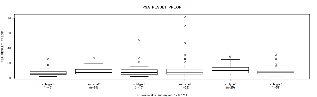
'MIRseq Mature cHierClus subtypes' versus 'PSA_VALUE'

P value = 0.379 (Kruskal-Wallis (anova)), Q value = 1

Table S149. Clustering Approach #10: 'MIRseq Mature cHierClus subtypes' versus Clinical Feature #13: 'PSA_VALUE'

	nPatients	Mean (Std.Dev)
ALL	193	0.7 (2.4)
subtype1	41	0.1 (0.2)
subtype2	24	0.1 (0.3)
subtype3	14	1.8 (3.9)
subtype4	43	0.9 (3.0)
subtype5	25	1.2 (3.8)
subtype6	46	0.5 (1.4)

Figure S139. Get High-res Image Clustering Approach #10: 'MIRseq Mature cHierClus subtypes' versus Clinical Feature #13: 'PSA_VALUE'

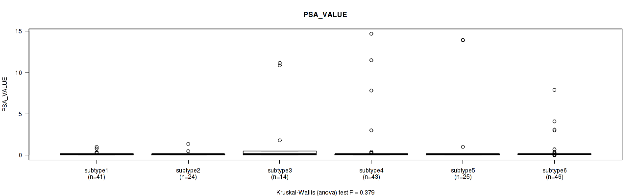
'MIRseq Mature cHierClus subtypes' versus 'RACE'

P value = 0.803 (Fisher's exact test), Q value = 1

Table S150. Clustering Approach #10: 'MIRseq Mature cHierClus subtypes' versus Clinical Feature #14: 'RACE'

nPatients	ASIAN	BLACK OR AFRICAN AMERICAN	WHITE
ALL	1	3	91
subtype1	0	0	5
subtype2	0	0	11
subtype3	0	0	3
subtype4	0	0	8
subtype5	0	0	25
subtype6	1	3	39

Figure S140. Get High-res Image Clustering Approach #10: 'MIRseq Mature cHierClus subtypes' versus Clinical Feature #14: 'RACE'

Methods & Data

Input

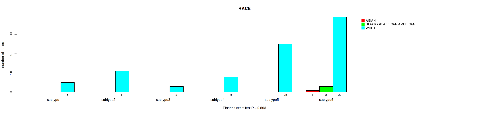
Cluster data file = PRAD-TP.mergedcluster.txt
Clinical data file = PRAD-TP.merged_data.txt
Number of patients = 367
Number of clustering approaches = 10
Number of selected clinical features = 14
Exclude small clusters that include fewer than K patients, K = 3

Clustering approaches

CNMF clustering

consensus non-negative matrix factorization clustering approach (Brunet et al. 2004)

Consensus hierarchical clustering

Resampling-based clustering method (Monti et al. 2003)

Survival analysis

For survival clinical features, the Kaplan-Meier survival curves of tumors with and without gene mutations were plotted and the statistical significance P values were estimated by logrank test (Bland and Altman 2004) using the 'survdiff' function in R

Fisher's exact test

For binary clinical features, two-tailed Fisher's exact tests (Fisher 1922) were used to estimate the P values using the 'fisher.test' function in R

Q value calculation

For multiple hypothesis correction, Q value is the False Discovery Rate (FDR) analogue of the P value (Benjamini and Hochberg 1995), defined as the minimum FDR at which the test may be called significant. We used the 'Benjamini and Hochberg' method of 'p.adjust' function in R to convert P values into Q values.

Download Results

In addition to the links below, the full results of the analysis summarized in this report can also be downloaded programmatically using firehose_get, or interactively from either the Broad GDAC website or TCGA Data Coordination Center Portal.

References

[1] Brunet et al., Metagenes and molecular pattern discovery using matrix factorization, PNAS 101(12):4164-9 (2004)

[2] Monti et al., Consensus Clustering: A Resampling-Based Method for Class Discovery and Visualization of Gene Expression Microarray Data, Machine Learning 52(1):91-118 (2003)

[3] Bland and Altman, Statistics notes: The logrank test, BMJ 328(7447):1073 (2004)

[4] Fisher, R.A., On the interpretation of chi-square from contingency tables, and the calculation of P, Journal of the Royal Statistical Society 85(1):87-94 (1922)

[5] Benjamini and Hochberg, Controlling the false discovery rate: a practical and powerful approach to multiple testing, Journal of the Royal Statistical Society Series B 59:289-300 (1995)

Made with Nozzle