This pipeline computes the correlation between cancer subtypes identified by different molecular patterns and selected clinical features.
Testing the association between subtypes identified by 8 different clustering approaches and 14 clinical features across 488 patients, 67 significant findings detected with P value < 0.05 and Q value < 0.25.
-
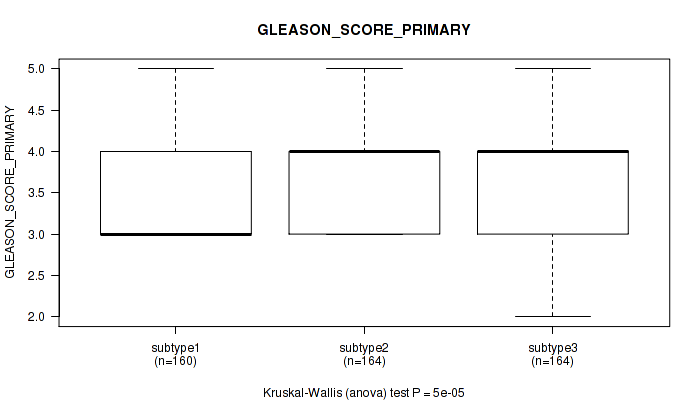
3 subtypes identified in current cancer cohort by 'Copy Number Ratio CNMF subtypes'. These subtypes correlate to 'YEARS_TO_BIRTH', 'PATHOLOGY_T_STAGE', 'PATHOLOGY_N_STAGE', 'COMPLETENESS_OF_RESECTION', 'NUMBER_OF_LYMPH_NODES', 'GLEASON_SCORE_COMBINED', 'GLEASON_SCORE_PRIMARY', 'GLEASON_SCORE_SECONDARY', 'GLEASON_SCORE', 'PSA_RESULT_PREOP', and 'PSA_VALUE'.
-
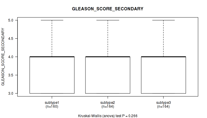
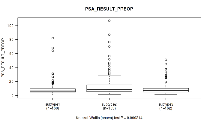
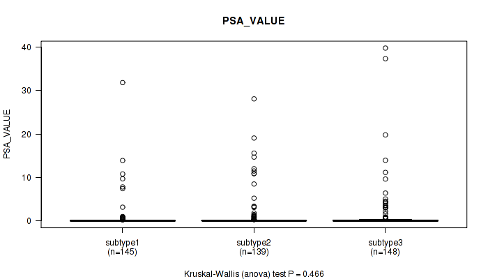
3 subtypes identified in current cancer cohort by 'METHLYATION CNMF'. These subtypes correlate to 'YEARS_TO_BIRTH', 'PATHOLOGY_T_STAGE', 'COMPLETENESS_OF_RESECTION', 'GLEASON_SCORE_COMBINED', 'GLEASON_SCORE_PRIMARY', 'GLEASON_SCORE', and 'PSA_RESULT_PREOP'.
-
CNMF clustering analysis on sequencing-based mRNA expression data identified 3 subtypes that correlate to 'PATHOLOGY_T_STAGE', 'NUMBER_OF_LYMPH_NODES', 'GLEASON_SCORE_COMBINED', 'GLEASON_SCORE_PRIMARY', 'GLEASON_SCORE', 'PSA_RESULT_PREOP', and 'PSA_VALUE'.
-
Consensus hierarchical clustering analysis on sequencing-based mRNA expression data identified 3 subtypes that correlate to 'YEARS_TO_BIRTH', 'PATHOLOGY_T_STAGE', 'COMPLETENESS_OF_RESECTION', 'NUMBER_OF_LYMPH_NODES', 'GLEASON_SCORE_COMBINED', 'GLEASON_SCORE_PRIMARY', 'GLEASON_SCORE', 'PSA_RESULT_PREOP', and 'RACE'.
-
3 subtypes identified in current cancer cohort by 'MIRSEQ CNMF'. These subtypes correlate to 'PATHOLOGY_T_STAGE', 'PATHOLOGY_N_STAGE', 'NUMBER_OF_LYMPH_NODES', 'GLEASON_SCORE_COMBINED', 'GLEASON_SCORE_PRIMARY', 'GLEASON_SCORE_SECONDARY', 'GLEASON_SCORE', and 'PSA_VALUE'.
-
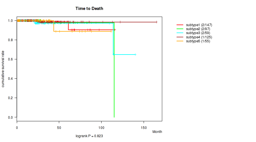
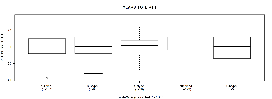
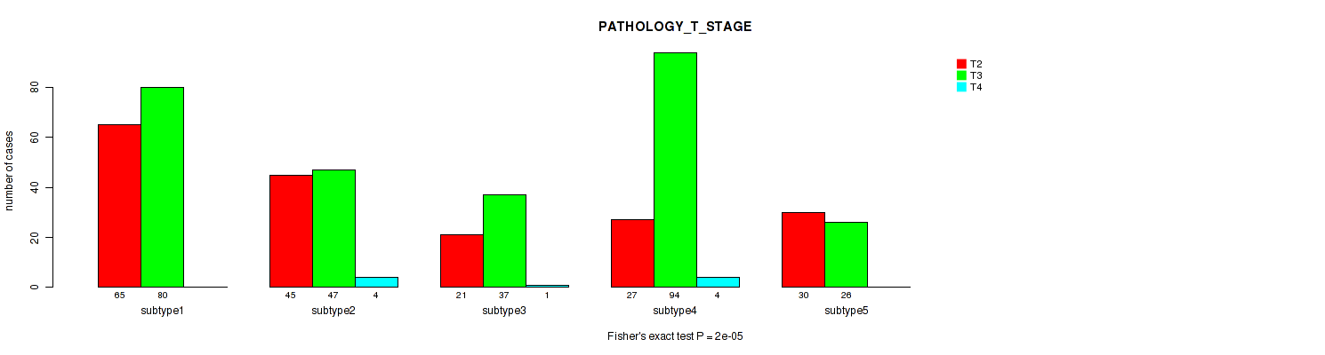
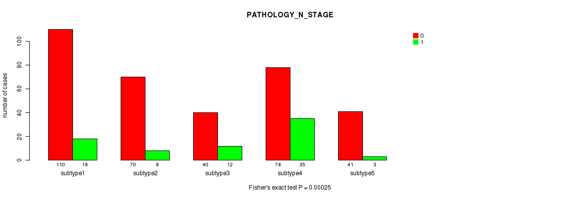
5 subtypes identified in current cancer cohort by 'MIRSEQ CHIERARCHICAL'. These subtypes correlate to 'YEARS_TO_BIRTH', 'PATHOLOGY_T_STAGE', 'PATHOLOGY_N_STAGE', 'COMPLETENESS_OF_RESECTION', 'NUMBER_OF_LYMPH_NODES', 'GLEASON_SCORE_COMBINED', 'GLEASON_SCORE_PRIMARY', 'GLEASON_SCORE_SECONDARY', and 'GLEASON_SCORE'.
-
4 subtypes identified in current cancer cohort by 'MIRseq Mature CNMF subtypes'. These subtypes correlate to 'YEARS_TO_BIRTH', 'PATHOLOGY_T_STAGE', 'COMPLETENESS_OF_RESECTION', 'GLEASON_SCORE_COMBINED', 'GLEASON_SCORE_PRIMARY', 'GLEASON_SCORE_SECONDARY', and 'GLEASON_SCORE'.
-
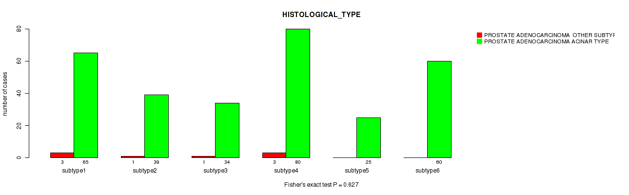
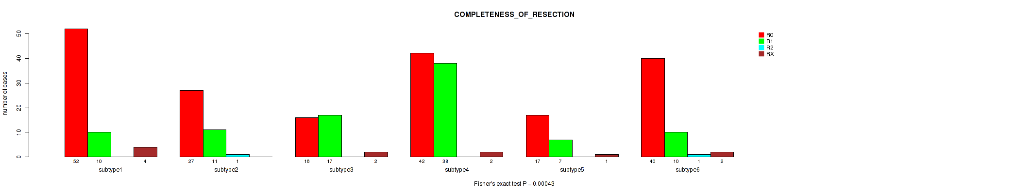
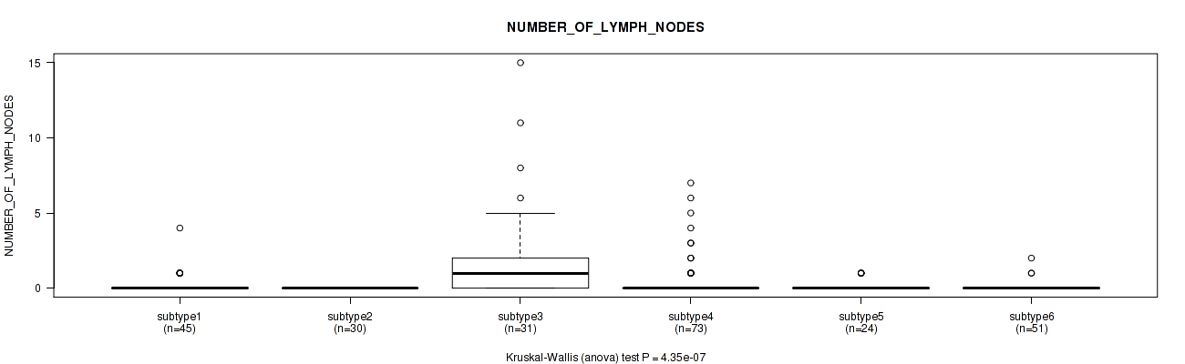
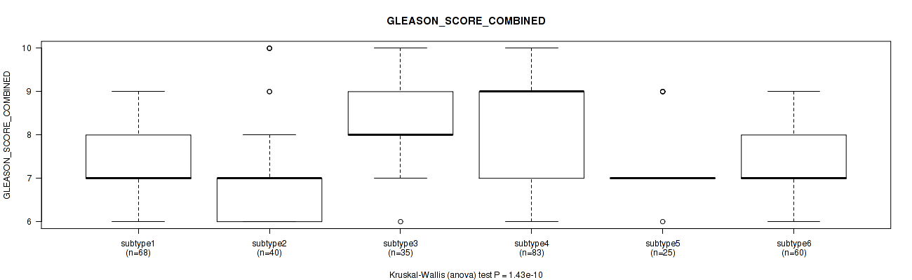
6 subtypes identified in current cancer cohort by 'MIRseq Mature cHierClus subtypes'. These subtypes correlate to 'YEARS_TO_BIRTH', 'PATHOLOGY_T_STAGE', 'PATHOLOGY_N_STAGE', 'COMPLETENESS_OF_RESECTION', 'NUMBER_OF_LYMPH_NODES', 'GLEASON_SCORE_COMBINED', 'GLEASON_SCORE_PRIMARY', 'GLEASON_SCORE_SECONDARY', and 'GLEASON_SCORE'.
Table 1. Get Full Table Overview of the association between subtypes identified by 8 different clustering approaches and 14 clinical features. Shown in the table are P values (Q values). Thresholded by P value < 0.05 and Q value < 0.25, 67 significant findings detected.
|
Clinical Features |
Statistical Tests |
Copy Number Ratio CNMF subtypes |
METHLYATION CNMF |
RNAseq CNMF subtypes |
RNAseq cHierClus subtypes |
MIRSEQ CNMF |
MIRSEQ CHIERARCHICAL |
MIRseq Mature CNMF subtypes |
MIRseq Mature cHierClus subtypes |
| Time to Death | logrank test |
0.907 (0.923) |
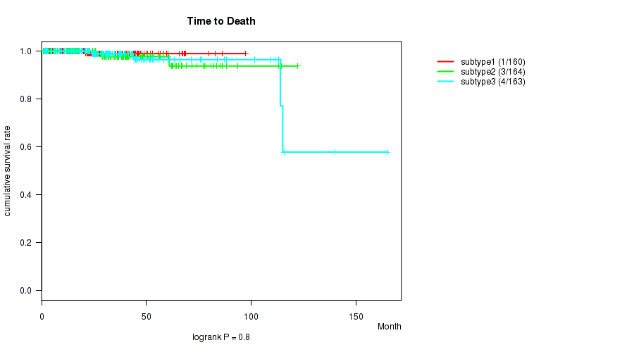
0.8 (0.834) |
0.375 (0.451) |
0.8 (0.834) |
0.614 (0.702) |
0.823 (0.846) |
0.721 (0.784) |
0.942 (0.95) |
| YEARS TO BIRTH | Kruskal-Wallis (anova) |
0.00146 (0.00379) |
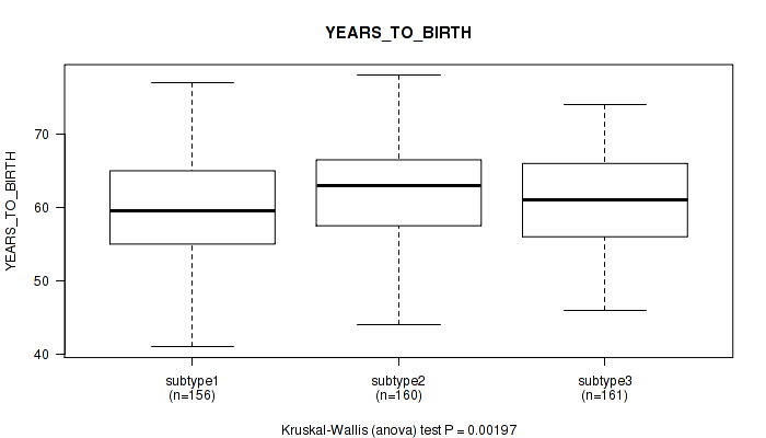
0.00197 (0.00501) |
0.144 (0.209) |
0.0169 (0.0343) |
0.132 (0.196) |
0.0401 (0.069) |
0.00962 (0.0203) |
0.0334 (0.0604) |
| PATHOLOGY T STAGE | Fisher's exact test |
1e-05 (5.89e-05) |
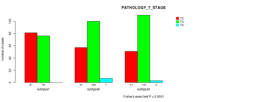
0.0001 (0.000373) |
0.00014 (0.000506) |
0.00364 (0.00867) |
0.00864 (0.0186) |
2e-05 (9.33e-05) |
0.00767 (0.0168) |
2e-05 (9.33e-05) |
| PATHOLOGY N STAGE | Fisher's exact test |
1e-05 (5.89e-05) |
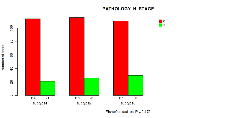
0.472 (0.557) |
0.0936 (0.146) |
0.0584 (0.0963) |
0.00636 (0.0142) |
0.00025 (0.000821) |
0.296 (0.381) |
2e-05 (9.33e-05) |
| HISTOLOGICAL TYPE | Fisher's exact test |
0.181 (0.253) |
0.675 (0.756) |
0.35 (0.43) |
0.229 (0.312) |
0.105 (0.159) |
0.782 (0.834) |
0.151 (0.216) |
0.627 (0.71) |
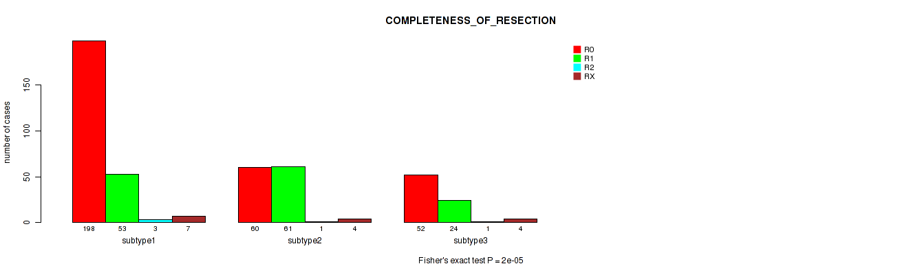
| COMPLETENESS OF RESECTION | Fisher's exact test |
2e-05 (9.33e-05) |
0.0319 (0.0595) |
0.104 (0.159) |
0.0247 (0.0478) |
0.172 (0.244) |
9e-05 (0.00035) |
0.0008 (0.00224) |
0.00043 (0.0013) |
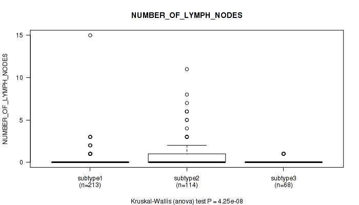
| NUMBER OF LYMPH NODES | Kruskal-Wallis (anova) |
4.25e-08 (4.77e-07) |
0.346 (0.43) |
0.0416 (0.0705) |
0.04 (0.069) |
0.00375 (0.00876) |
3.2e-05 (0.000141) |
0.344 (0.43) |
4.35e-07 (4.42e-06) |
| GLEASON SCORE COMBINED | Kruskal-Wallis (anova) |
2.87e-18 (1.61e-16) |
0.000257 (0.000821) |
0.0217 (0.0434) |
0.000174 (0.00061) |
4.68e-06 (3.67e-05) |
7.95e-12 (2.22e-10) |
3.49e-06 (3.01e-05) |
1.43e-10 (2.28e-09) |
| GLEASON SCORE PRIMARY | Kruskal-Wallis (anova) |
8.52e-18 (3.18e-16) |
5e-05 (0.000207) |
0.00264 (0.00642) |
8.75e-06 (5.76e-05) |
9.07e-05 (0.00035) |
1.07e-08 (1.33e-07) |
1.42e-05 (7.93e-05) |
7.2e-09 (1.01e-07) |
| GLEASON SCORE SECONDARY | Kruskal-Wallis (anova) |
3.28e-05 (0.000141) |
0.266 (0.355) |
0.0627 (0.102) |
0.25 (0.338) |
0.00559 (0.0128) |
0.000515 (0.00148) |
0.0121 (0.0251) |
0.000405 (0.00126) |
| GLEASON SCORE | Kruskal-Wallis (anova) |
2.48e-22 (2.78e-20) |
0.000493 (0.00145) |
0.000835 (0.00228) |
8.31e-06 (5.76e-05) |
4.92e-06 (3.67e-05) |
7.15e-11 (1.6e-09) |
9.56e-07 (8.93e-06) |
1.27e-10 (2.28e-09) |
| PSA RESULT PREOP | Kruskal-Wallis (anova) |
0.00213 (0.00531) |
0.000214 (0.000728) |
0.00117 (0.00311) |
0.0312 (0.0593) |
0.0918 (0.145) |
0.294 (0.381) |
0.295 (0.381) |
0.134 (0.197) |
| PSA VALUE | Kruskal-Wallis (anova) |
0.0326 (0.0598) |
0.466 (0.555) |
0.0433 (0.0723) |
0.554 (0.646) |
0.0389 (0.069) |
0.684 (0.758) |
0.0734 (0.117) |
0.363 (0.442) |
| RACE | Fisher's exact test |
0.564 (0.652) |
1 (1.00) |
0.337 (0.429) |
0.0226 (0.0445) |
0.215 (0.297) |
0.708 (0.777) |
0.805 (0.834) |
0.804 (0.834) |
Table S1. Description of clustering approach #1: 'Copy Number Ratio CNMF subtypes'
| Cluster Labels | 1 | 2 | 3 |
|---|---|---|---|
| Number of samples | 269 | 128 | 85 |
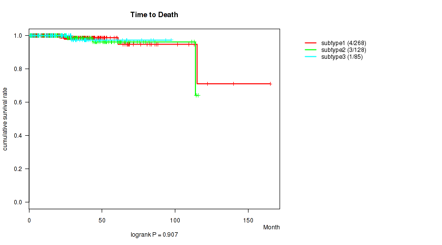
P value = 0.907 (logrank test), Q value = 0.92
Table S2. Clustering Approach #1: 'Copy Number Ratio CNMF subtypes' versus Clinical Feature #1: 'Time to Death'
| nPatients | nDeath | Duration Range (Median), Month | |
|---|---|---|---|
| ALL | 481 | 8 | 0.7 - 165.2 (26.7) |
| subtype1 | 268 | 4 | 0.7 - 165.2 (26.2) |
| subtype2 | 128 | 3 | 0.8 - 115.9 (28.3) |
| subtype3 | 85 | 1 | 1.0 - 97.4 (25.5) |
Figure S1. Get High-res Image Clustering Approach #1: 'Copy Number Ratio CNMF subtypes' versus Clinical Feature #1: 'Time to Death'
P value = 0.00146 (Kruskal-Wallis (anova)), Q value = 0.0038
Table S3. Clustering Approach #1: 'Copy Number Ratio CNMF subtypes' versus Clinical Feature #2: 'YEARS_TO_BIRTH'
| nPatients | Mean (Std.Dev) | |
|---|---|---|
| ALL | 471 | 60.9 (6.8) |
| subtype1 | 263 | 60.1 (6.8) |
| subtype2 | 125 | 62.7 (6.2) |
| subtype3 | 83 | 60.7 (7.4) |
Figure S2. Get High-res Image Clustering Approach #1: 'Copy Number Ratio CNMF subtypes' versus Clinical Feature #2: 'YEARS_TO_BIRTH'

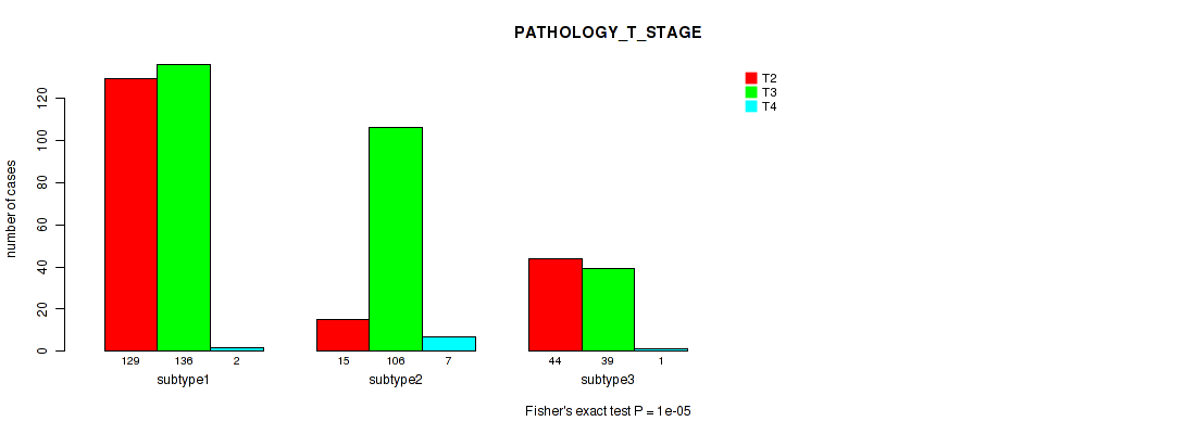
P value = 1e-05 (Fisher's exact test), Q value = 5.9e-05
Table S4. Clustering Approach #1: 'Copy Number Ratio CNMF subtypes' versus Clinical Feature #3: 'PATHOLOGY_T_STAGE'
| nPatients | T2 | T3 | T4 |
|---|---|---|---|
| ALL | 188 | 281 | 10 |
| subtype1 | 129 | 136 | 2 |
| subtype2 | 15 | 106 | 7 |
| subtype3 | 44 | 39 | 1 |
Figure S3. Get High-res Image Clustering Approach #1: 'Copy Number Ratio CNMF subtypes' versus Clinical Feature #3: 'PATHOLOGY_T_STAGE'
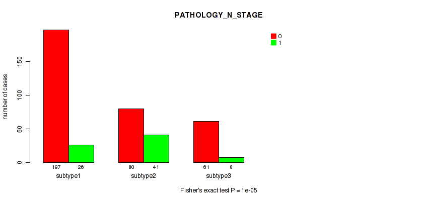
P value = 1e-05 (Fisher's exact test), Q value = 5.9e-05
Table S5. Clustering Approach #1: 'Copy Number Ratio CNMF subtypes' versus Clinical Feature #4: 'PATHOLOGY_N_STAGE'
| nPatients | 0 | 1 |
|---|---|---|
| ALL | 338 | 75 |
| subtype1 | 197 | 26 |
| subtype2 | 80 | 41 |
| subtype3 | 61 | 8 |
Figure S4. Get High-res Image Clustering Approach #1: 'Copy Number Ratio CNMF subtypes' versus Clinical Feature #4: 'PATHOLOGY_N_STAGE'
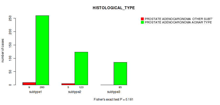
P value = 0.181 (Fisher's exact test), Q value = 0.25
Table S6. Clustering Approach #1: 'Copy Number Ratio CNMF subtypes' versus Clinical Feature #5: 'HISTOLOGICAL_TYPE'
| nPatients | PROSTATE ADENOCARCINOMA OTHER SUBTYPE | PROSTATE ADENOCARCINOMA ACINAR TYPE |
|---|---|---|
| ALL | 14 | 468 |
| subtype1 | 9 | 260 |
| subtype2 | 5 | 123 |
| subtype3 | 0 | 85 |
Figure S5. Get High-res Image Clustering Approach #1: 'Copy Number Ratio CNMF subtypes' versus Clinical Feature #5: 'HISTOLOGICAL_TYPE'
P value = 2e-05 (Fisher's exact test), Q value = 9.3e-05
Table S7. Clustering Approach #1: 'Copy Number Ratio CNMF subtypes' versus Clinical Feature #6: 'COMPLETENESS_OF_RESECTION'
| nPatients | R0 | R1 | R2 | RX |
|---|---|---|---|---|
| ALL | 310 | 138 | 5 | 15 |
| subtype1 | 198 | 53 | 3 | 7 |
| subtype2 | 60 | 61 | 1 | 4 |
| subtype3 | 52 | 24 | 1 | 4 |
Figure S6. Get High-res Image Clustering Approach #1: 'Copy Number Ratio CNMF subtypes' versus Clinical Feature #6: 'COMPLETENESS_OF_RESECTION'
P value = 4.25e-08 (Kruskal-Wallis (anova)), Q value = 4.8e-07
Table S8. Clustering Approach #1: 'Copy Number Ratio CNMF subtypes' versus Clinical Feature #7: 'NUMBER_OF_LYMPH_NODES'
| nPatients | Mean (Std.Dev) | |
|---|---|---|
| ALL | 395 | 0.4 (1.4) |
| subtype1 | 213 | 0.2 (1.1) |
| subtype2 | 114 | 1.0 (1.9) |
| subtype3 | 68 | 0.1 (0.3) |
Figure S7. Get High-res Image Clustering Approach #1: 'Copy Number Ratio CNMF subtypes' versus Clinical Feature #7: 'NUMBER_OF_LYMPH_NODES'
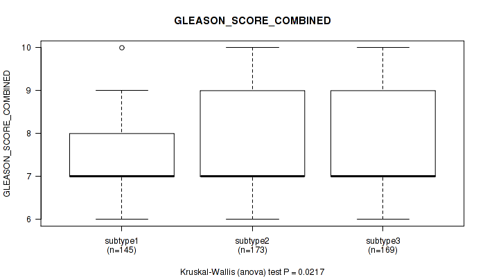
P value = 2.87e-18 (Kruskal-Wallis (anova)), Q value = 1.6e-16
Table S9. Clustering Approach #1: 'Copy Number Ratio CNMF subtypes' versus Clinical Feature #8: 'GLEASON_SCORE_COMBINED'
| nPatients | Mean (Std.Dev) | |
|---|---|---|
| ALL | 482 | 7.6 (1.0) |
| subtype1 | 269 | 7.3 (0.9) |
| subtype2 | 128 | 8.2 (1.0) |
| subtype3 | 85 | 7.4 (0.9) |
Figure S8. Get High-res Image Clustering Approach #1: 'Copy Number Ratio CNMF subtypes' versus Clinical Feature #8: 'GLEASON_SCORE_COMBINED'

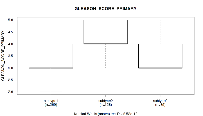
P value = 8.52e-18 (Kruskal-Wallis (anova)), Q value = 3.2e-16
Table S10. Clustering Approach #1: 'Copy Number Ratio CNMF subtypes' versus Clinical Feature #9: 'GLEASON_SCORE_PRIMARY'
| nPatients | Mean (Std.Dev) | |
|---|---|---|
| ALL | 482 | 3.7 (0.7) |
| subtype1 | 269 | 3.5 (0.6) |
| subtype2 | 128 | 4.1 (0.6) |
| subtype3 | 85 | 3.5 (0.6) |
Figure S9. Get High-res Image Clustering Approach #1: 'Copy Number Ratio CNMF subtypes' versus Clinical Feature #9: 'GLEASON_SCORE_PRIMARY'
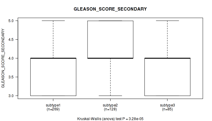
P value = 3.28e-05 (Kruskal-Wallis (anova)), Q value = 0.00014
Table S11. Clustering Approach #1: 'Copy Number Ratio CNMF subtypes' versus Clinical Feature #10: 'GLEASON_SCORE_SECONDARY'
| nPatients | Mean (Std.Dev) | |
|---|---|---|
| ALL | 482 | 3.9 (0.7) |
| subtype1 | 269 | 3.8 (0.7) |
| subtype2 | 128 | 4.1 (0.7) |
| subtype3 | 85 | 3.8 (0.6) |
Figure S10. Get High-res Image Clustering Approach #1: 'Copy Number Ratio CNMF subtypes' versus Clinical Feature #10: 'GLEASON_SCORE_SECONDARY'
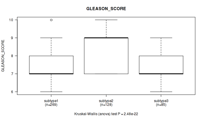
P value = 2.48e-22 (Kruskal-Wallis (anova)), Q value = 2.8e-20
Table S12. Clustering Approach #1: 'Copy Number Ratio CNMF subtypes' versus Clinical Feature #11: 'GLEASON_SCORE'
| nPatients | Mean (Std.Dev) | |
|---|---|---|
| ALL | 482 | 7.6 (1.0) |
| subtype1 | 269 | 7.3 (0.9) |
| subtype2 | 128 | 8.4 (0.9) |
| subtype3 | 85 | 7.4 (0.9) |
Figure S11. Get High-res Image Clustering Approach #1: 'Copy Number Ratio CNMF subtypes' versus Clinical Feature #11: 'GLEASON_SCORE'
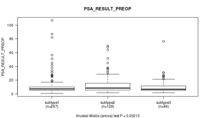
P value = 0.00213 (Kruskal-Wallis (anova)), Q value = 0.0053
Table S13. Clustering Approach #1: 'Copy Number Ratio CNMF subtypes' versus Clinical Feature #12: 'PSA_RESULT_PREOP'
| nPatients | Mean (Std.Dev) | |
|---|---|---|
| ALL | 479 | 10.8 (11.7) |
| subtype1 | 267 | 9.8 (11.5) |
| subtype2 | 128 | 13.3 (12.7) |
| subtype3 | 84 | 10.2 (9.9) |
Figure S12. Get High-res Image Clustering Approach #1: 'Copy Number Ratio CNMF subtypes' versus Clinical Feature #12: 'PSA_RESULT_PREOP'
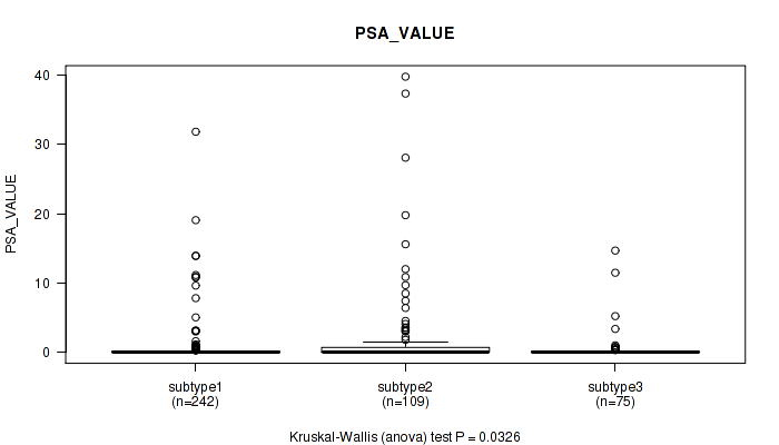
P value = 0.0326 (Kruskal-Wallis (anova)), Q value = 0.06
Table S14. Clustering Approach #1: 'Copy Number Ratio CNMF subtypes' versus Clinical Feature #13: 'PSA_VALUE'
| nPatients | Mean (Std.Dev) | |
|---|---|---|
| ALL | 426 | 1.1 (4.1) |
| subtype1 | 242 | 0.7 (3.0) |
| subtype2 | 109 | 2.2 (6.5) |
| subtype3 | 75 | 0.6 (2.2) |
Figure S13. Get High-res Image Clustering Approach #1: 'Copy Number Ratio CNMF subtypes' versus Clinical Feature #13: 'PSA_VALUE'
P value = 0.564 (Fisher's exact test), Q value = 0.65
Table S15. Clustering Approach #1: 'Copy Number Ratio CNMF subtypes' versus Clinical Feature #14: 'RACE'
| nPatients | ASIAN | BLACK OR AFRICAN AMERICAN | WHITE |
|---|---|---|---|
| ALL | 2 | 7 | 146 |
| subtype1 | 2 | 3 | 90 |
| subtype2 | 0 | 1 | 29 |
| subtype3 | 0 | 3 | 27 |
Figure S14. Get High-res Image Clustering Approach #1: 'Copy Number Ratio CNMF subtypes' versus Clinical Feature #14: 'RACE'
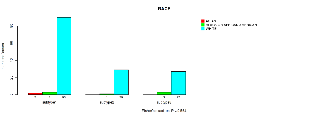
Table S16. Description of clustering approach #2: 'METHLYATION CNMF'
| Cluster Labels | 1 | 2 | 3 |
|---|---|---|---|
| Number of samples | 160 | 164 | 164 |
P value = 0.8 (logrank test), Q value = 0.83
Table S17. Clustering Approach #2: 'METHLYATION CNMF' versus Clinical Feature #1: 'Time to Death'
| nPatients | nDeath | Duration Range (Median), Month | |
|---|---|---|---|
| ALL | 487 | 8 | 0.7 - 165.2 (26.4) |
| subtype1 | 160 | 1 | 1.0 - 97.4 (24.8) |
| subtype2 | 164 | 3 | 0.7 - 122.2 (28.7) |
| subtype3 | 163 | 4 | 1.0 - 165.2 (25.9) |
Figure S15. Get High-res Image Clustering Approach #2: 'METHLYATION CNMF' versus Clinical Feature #1: 'Time to Death'
P value = 0.00197 (Kruskal-Wallis (anova)), Q value = 0.005
Table S18. Clustering Approach #2: 'METHLYATION CNMF' versus Clinical Feature #2: 'YEARS_TO_BIRTH'
| nPatients | Mean (Std.Dev) | |
|---|---|---|
| ALL | 477 | 60.9 (6.8) |
| subtype1 | 156 | 59.8 (6.9) |
| subtype2 | 160 | 62.4 (6.9) |
| subtype3 | 161 | 60.5 (6.4) |
Figure S16. Get High-res Image Clustering Approach #2: 'METHLYATION CNMF' versus Clinical Feature #2: 'YEARS_TO_BIRTH'
P value = 1e-04 (Fisher's exact test), Q value = 0.00037
Table S19. Clustering Approach #2: 'METHLYATION CNMF' versus Clinical Feature #3: 'PATHOLOGY_T_STAGE'
| nPatients | T2 | T3 | T4 |
|---|---|---|---|
| ALL | 189 | 286 | 10 |
| subtype1 | 81 | 76 | 0 |
| subtype2 | 57 | 100 | 7 |
| subtype3 | 51 | 110 | 3 |
Figure S17. Get High-res Image Clustering Approach #2: 'METHLYATION CNMF' versus Clinical Feature #3: 'PATHOLOGY_T_STAGE'
P value = 0.472 (Fisher's exact test), Q value = 0.56
Table S20. Clustering Approach #2: 'METHLYATION CNMF' versus Clinical Feature #4: 'PATHOLOGY_N_STAGE'
| nPatients | 0 | 1 |
|---|---|---|
| ALL | 341 | 77 |
| subtype1 | 114 | 21 |
| subtype2 | 116 | 26 |
| subtype3 | 111 | 30 |
Figure S18. Get High-res Image Clustering Approach #2: 'METHLYATION CNMF' versus Clinical Feature #4: 'PATHOLOGY_N_STAGE'
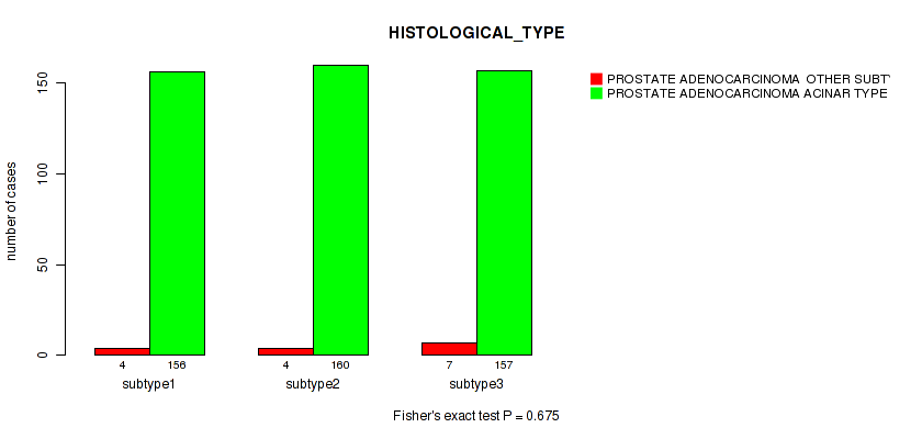
P value = 0.675 (Fisher's exact test), Q value = 0.76
Table S21. Clustering Approach #2: 'METHLYATION CNMF' versus Clinical Feature #5: 'HISTOLOGICAL_TYPE'
| nPatients | PROSTATE ADENOCARCINOMA OTHER SUBTYPE | PROSTATE ADENOCARCINOMA ACINAR TYPE |
|---|---|---|
| ALL | 15 | 473 |
| subtype1 | 4 | 156 |
| subtype2 | 4 | 160 |
| subtype3 | 7 | 157 |
Figure S19. Get High-res Image Clustering Approach #2: 'METHLYATION CNMF' versus Clinical Feature #5: 'HISTOLOGICAL_TYPE'
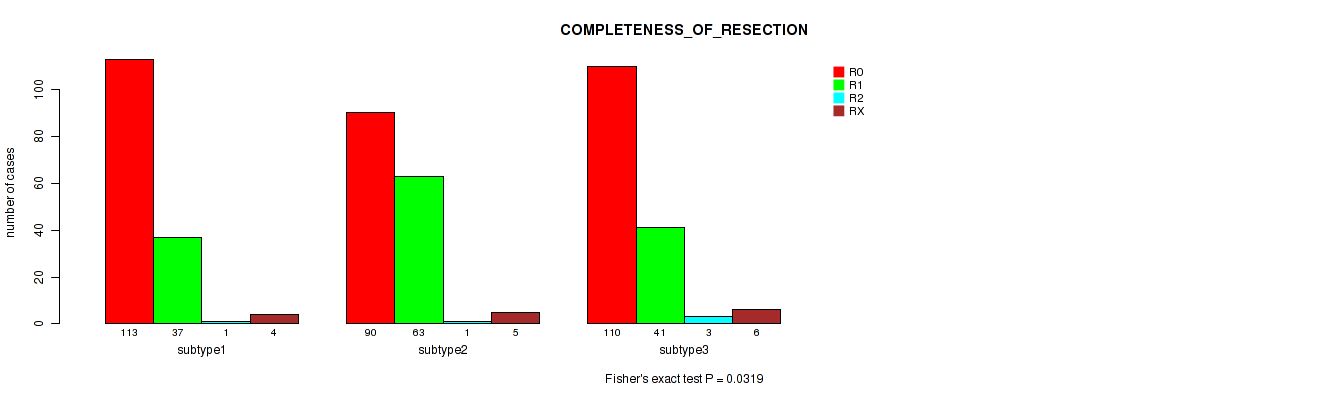
P value = 0.0319 (Fisher's exact test), Q value = 0.06
Table S22. Clustering Approach #2: 'METHLYATION CNMF' versus Clinical Feature #6: 'COMPLETENESS_OF_RESECTION'
| nPatients | R0 | R1 | R2 | RX |
|---|---|---|---|---|
| ALL | 313 | 141 | 5 | 15 |
| subtype1 | 113 | 37 | 1 | 4 |
| subtype2 | 90 | 63 | 1 | 5 |
| subtype3 | 110 | 41 | 3 | 6 |
Figure S20. Get High-res Image Clustering Approach #2: 'METHLYATION CNMF' versus Clinical Feature #6: 'COMPLETENESS_OF_RESECTION'
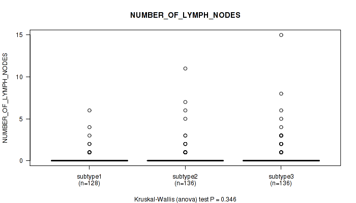
P value = 0.346 (Kruskal-Wallis (anova)), Q value = 0.43
Table S23. Clustering Approach #2: 'METHLYATION CNMF' versus Clinical Feature #7: 'NUMBER_OF_LYMPH_NODES'
| nPatients | Mean (Std.Dev) | |
|---|---|---|
| ALL | 400 | 0.4 (1.4) |
| subtype1 | 128 | 0.3 (0.8) |
| subtype2 | 136 | 0.4 (1.4) |
| subtype3 | 136 | 0.6 (1.8) |
Figure S21. Get High-res Image Clustering Approach #2: 'METHLYATION CNMF' versus Clinical Feature #7: 'NUMBER_OF_LYMPH_NODES'
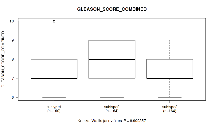
P value = 0.000257 (Kruskal-Wallis (anova)), Q value = 0.00082
Table S24. Clustering Approach #2: 'METHLYATION CNMF' versus Clinical Feature #8: 'GLEASON_SCORE_COMBINED'
| nPatients | Mean (Std.Dev) | |
|---|---|---|
| ALL | 488 | 7.6 (1.0) |
| subtype1 | 160 | 7.4 (1.0) |
| subtype2 | 164 | 7.8 (1.0) |
| subtype3 | 164 | 7.5 (1.0) |
Figure S22. Get High-res Image Clustering Approach #2: 'METHLYATION CNMF' versus Clinical Feature #8: 'GLEASON_SCORE_COMBINED'
P value = 5e-05 (Kruskal-Wallis (anova)), Q value = 0.00021
Table S25. Clustering Approach #2: 'METHLYATION CNMF' versus Clinical Feature #9: 'GLEASON_SCORE_PRIMARY'
| nPatients | Mean (Std.Dev) | |
|---|---|---|
| ALL | 488 | 3.7 (0.7) |
| subtype1 | 160 | 3.6 (0.7) |
| subtype2 | 164 | 3.9 (0.7) |
| subtype3 | 164 | 3.6 (0.6) |
Figure S23. Get High-res Image Clustering Approach #2: 'METHLYATION CNMF' versus Clinical Feature #9: 'GLEASON_SCORE_PRIMARY'
P value = 0.266 (Kruskal-Wallis (anova)), Q value = 0.36
Table S26. Clustering Approach #2: 'METHLYATION CNMF' versus Clinical Feature #10: 'GLEASON_SCORE_SECONDARY'
| nPatients | Mean (Std.Dev) | |
|---|---|---|
| ALL | 488 | 3.9 (0.7) |
| subtype1 | 160 | 3.8 (0.6) |
| subtype2 | 164 | 3.9 (0.7) |
| subtype3 | 164 | 3.9 (0.7) |
Figure S24. Get High-res Image Clustering Approach #2: 'METHLYATION CNMF' versus Clinical Feature #10: 'GLEASON_SCORE_SECONDARY'
P value = 0.000493 (Kruskal-Wallis (anova)), Q value = 0.0015
Table S27. Clustering Approach #2: 'METHLYATION CNMF' versus Clinical Feature #11: 'GLEASON_SCORE'
| nPatients | Mean (Std.Dev) | |
|---|---|---|
| ALL | 488 | 7.6 (1.0) |
| subtype1 | 160 | 7.4 (1.0) |
| subtype2 | 164 | 7.8 (1.0) |
| subtype3 | 164 | 7.6 (1.0) |
Figure S25. Get High-res Image Clustering Approach #2: 'METHLYATION CNMF' versus Clinical Feature #11: 'GLEASON_SCORE'

P value = 0.000214 (Kruskal-Wallis (anova)), Q value = 0.00073
Table S28. Clustering Approach #2: 'METHLYATION CNMF' versus Clinical Feature #12: 'PSA_RESULT_PREOP'
| nPatients | Mean (Std.Dev) | |
|---|---|---|
| ALL | 485 | 10.8 (11.7) |
| subtype1 | 160 | 9.0 (10.1) |
| subtype2 | 163 | 13.8 (15.2) |
| subtype3 | 162 | 9.7 (8.0) |
Figure S26. Get High-res Image Clustering Approach #2: 'METHLYATION CNMF' versus Clinical Feature #12: 'PSA_RESULT_PREOP'
P value = 0.466 (Kruskal-Wallis (anova)), Q value = 0.56
Table S29. Clustering Approach #2: 'METHLYATION CNMF' versus Clinical Feature #13: 'PSA_VALUE'
| nPatients | Mean (Std.Dev) | |
|---|---|---|
| ALL | 432 | 1.1 (4.1) |
| subtype1 | 145 | 0.7 (3.2) |
| subtype2 | 139 | 1.2 (3.9) |
| subtype3 | 148 | 1.3 (5.0) |
Figure S27. Get High-res Image Clustering Approach #2: 'METHLYATION CNMF' versus Clinical Feature #13: 'PSA_VALUE'
P value = 1 (Fisher's exact test), Q value = 1
Table S30. Clustering Approach #2: 'METHLYATION CNMF' versus Clinical Feature #14: 'RACE'
| nPatients | ASIAN | BLACK OR AFRICAN AMERICAN | WHITE |
|---|---|---|---|
| ALL | 2 | 7 | 147 |
| subtype1 | 1 | 2 | 53 |
| subtype2 | 0 | 2 | 37 |
| subtype3 | 1 | 3 | 57 |
Figure S28. Get High-res Image Clustering Approach #2: 'METHLYATION CNMF' versus Clinical Feature #14: 'RACE'
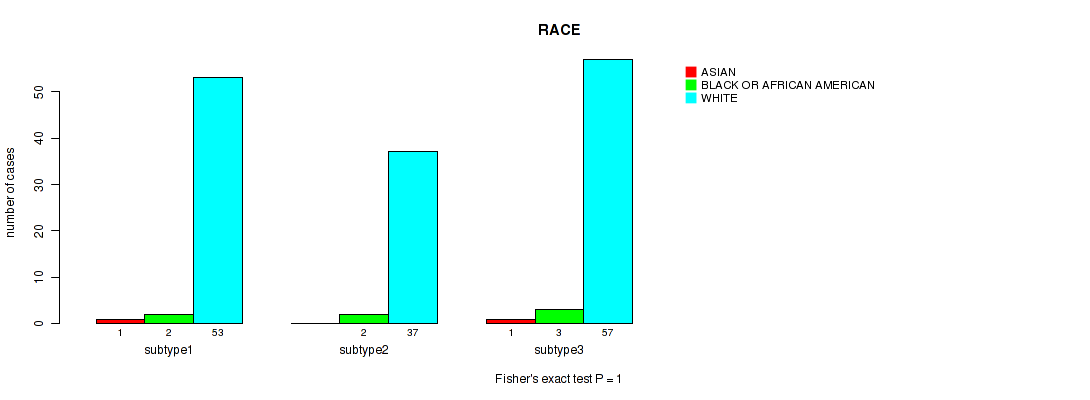
Table S31. Description of clustering approach #3: 'RNAseq CNMF subtypes'
| Cluster Labels | 1 | 2 | 3 |
|---|---|---|---|
| Number of samples | 145 | 173 | 169 |
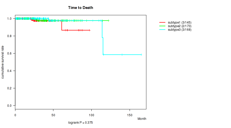
P value = 0.375 (logrank test), Q value = 0.45
Table S32. Clustering Approach #3: 'RNAseq CNMF subtypes' versus Clinical Feature #1: 'Time to Death'
| nPatients | nDeath | Duration Range (Median), Month | |
|---|---|---|---|
| ALL | 486 | 8 | 0.7 - 165.2 (26.5) |
| subtype1 | 145 | 3 | 0.7 - 97.4 (24.0) |
| subtype2 | 173 | 2 | 0.8 - 122.2 (28.2) |
| subtype3 | 168 | 3 | 0.9 - 165.2 (26.4) |
Figure S29. Get High-res Image Clustering Approach #3: 'RNAseq CNMF subtypes' versus Clinical Feature #1: 'Time to Death'
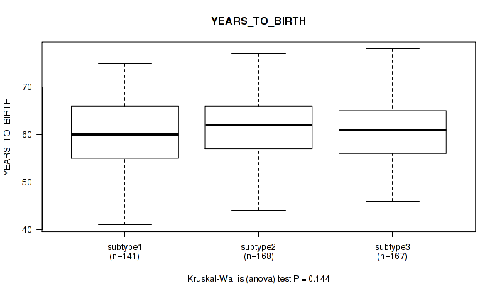
P value = 0.144 (Kruskal-Wallis (anova)), Q value = 0.21
Table S33. Clustering Approach #3: 'RNAseq CNMF subtypes' versus Clinical Feature #2: 'YEARS_TO_BIRTH'
| nPatients | Mean (Std.Dev) | |
|---|---|---|
| ALL | 476 | 60.9 (6.8) |
| subtype1 | 141 | 60.1 (7.2) |
| subtype2 | 168 | 61.8 (6.9) |
| subtype3 | 167 | 60.8 (6.4) |
Figure S30. Get High-res Image Clustering Approach #3: 'RNAseq CNMF subtypes' versus Clinical Feature #2: 'YEARS_TO_BIRTH'
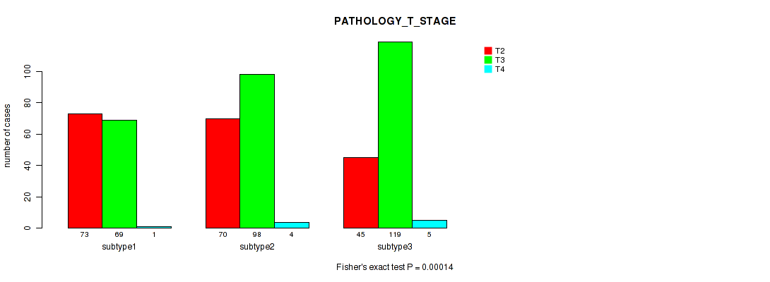
P value = 0.00014 (Fisher's exact test), Q value = 0.00051
Table S34. Clustering Approach #3: 'RNAseq CNMF subtypes' versus Clinical Feature #3: 'PATHOLOGY_T_STAGE'
| nPatients | T2 | T3 | T4 |
|---|---|---|---|
| ALL | 188 | 286 | 10 |
| subtype1 | 73 | 69 | 1 |
| subtype2 | 70 | 98 | 4 |
| subtype3 | 45 | 119 | 5 |
Figure S31. Get High-res Image Clustering Approach #3: 'RNAseq CNMF subtypes' versus Clinical Feature #3: 'PATHOLOGY_T_STAGE'
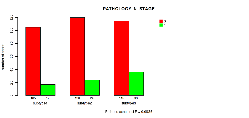
P value = 0.0936 (Fisher's exact test), Q value = 0.15
Table S35. Clustering Approach #3: 'RNAseq CNMF subtypes' versus Clinical Feature #4: 'PATHOLOGY_N_STAGE'
| nPatients | 0 | 1 |
|---|---|---|
| ALL | 340 | 77 |
| subtype1 | 105 | 17 |
| subtype2 | 120 | 24 |
| subtype3 | 115 | 36 |
Figure S32. Get High-res Image Clustering Approach #3: 'RNAseq CNMF subtypes' versus Clinical Feature #4: 'PATHOLOGY_N_STAGE'
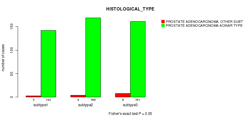
P value = 0.35 (Fisher's exact test), Q value = 0.43
Table S36. Clustering Approach #3: 'RNAseq CNMF subtypes' versus Clinical Feature #5: 'HISTOLOGICAL_TYPE'
| nPatients | PROSTATE ADENOCARCINOMA OTHER SUBTYPE | PROSTATE ADENOCARCINOMA ACINAR TYPE |
|---|---|---|
| ALL | 15 | 472 |
| subtype1 | 3 | 142 |
| subtype2 | 4 | 169 |
| subtype3 | 8 | 161 |
Figure S33. Get High-res Image Clustering Approach #3: 'RNAseq CNMF subtypes' versus Clinical Feature #5: 'HISTOLOGICAL_TYPE'
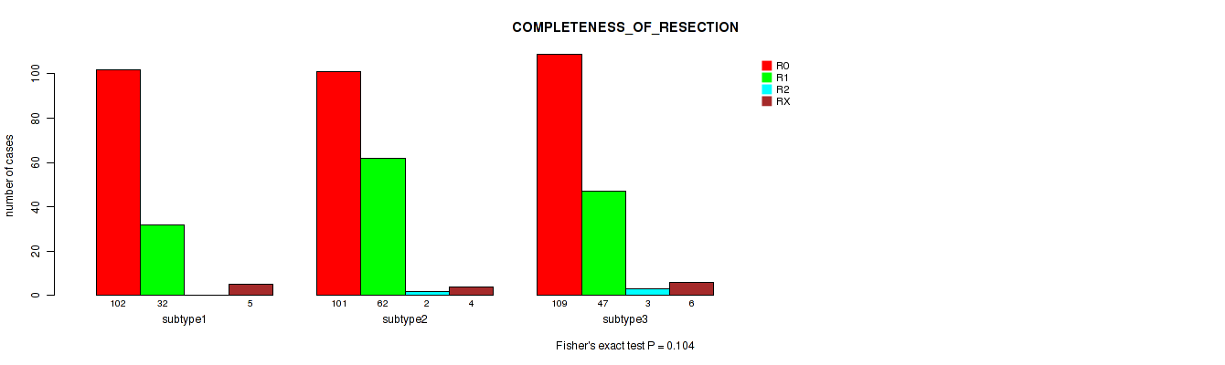
P value = 0.104 (Fisher's exact test), Q value = 0.16
Table S37. Clustering Approach #3: 'RNAseq CNMF subtypes' versus Clinical Feature #6: 'COMPLETENESS_OF_RESECTION'
| nPatients | R0 | R1 | R2 | RX |
|---|---|---|---|---|
| ALL | 312 | 141 | 5 | 15 |
| subtype1 | 102 | 32 | 0 | 5 |
| subtype2 | 101 | 62 | 2 | 4 |
| subtype3 | 109 | 47 | 3 | 6 |
Figure S34. Get High-res Image Clustering Approach #3: 'RNAseq CNMF subtypes' versus Clinical Feature #6: 'COMPLETENESS_OF_RESECTION'
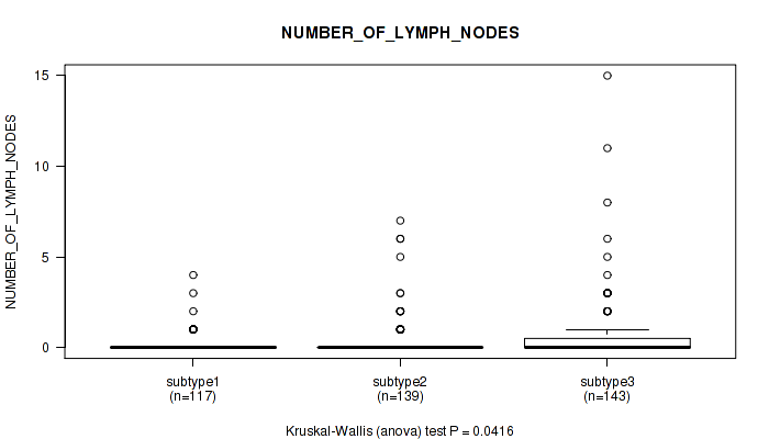
P value = 0.0416 (Kruskal-Wallis (anova)), Q value = 0.071
Table S38. Clustering Approach #3: 'RNAseq CNMF subtypes' versus Clinical Feature #7: 'NUMBER_OF_LYMPH_NODES'
| nPatients | Mean (Std.Dev) | |
|---|---|---|
| ALL | 399 | 0.4 (1.4) |
| subtype1 | 117 | 0.2 (0.6) |
| subtype2 | 139 | 0.4 (1.1) |
| subtype3 | 143 | 0.7 (1.9) |
Figure S35. Get High-res Image Clustering Approach #3: 'RNAseq CNMF subtypes' versus Clinical Feature #7: 'NUMBER_OF_LYMPH_NODES'
P value = 0.0217 (Kruskal-Wallis (anova)), Q value = 0.043
Table S39. Clustering Approach #3: 'RNAseq CNMF subtypes' versus Clinical Feature #8: 'GLEASON_SCORE_COMBINED'
| nPatients | Mean (Std.Dev) | |
|---|---|---|
| ALL | 487 | 7.6 (1.0) |
| subtype1 | 145 | 7.4 (0.9) |
| subtype2 | 173 | 7.6 (1.1) |
| subtype3 | 169 | 7.7 (1.0) |
Figure S36. Get High-res Image Clustering Approach #3: 'RNAseq CNMF subtypes' versus Clinical Feature #8: 'GLEASON_SCORE_COMBINED'
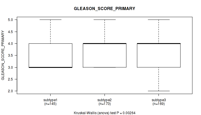
P value = 0.00264 (Kruskal-Wallis (anova)), Q value = 0.0064
Table S40. Clustering Approach #3: 'RNAseq CNMF subtypes' versus Clinical Feature #9: 'GLEASON_SCORE_PRIMARY'
| nPatients | Mean (Std.Dev) | |
|---|---|---|
| ALL | 487 | 3.7 (0.7) |
| subtype1 | 145 | 3.5 (0.7) |
| subtype2 | 173 | 3.8 (0.7) |
| subtype3 | 169 | 3.7 (0.6) |
Figure S37. Get High-res Image Clustering Approach #3: 'RNAseq CNMF subtypes' versus Clinical Feature #9: 'GLEASON_SCORE_PRIMARY'
P value = 0.0627 (Kruskal-Wallis (anova)), Q value = 0.1
Table S41. Clustering Approach #3: 'RNAseq CNMF subtypes' versus Clinical Feature #10: 'GLEASON_SCORE_SECONDARY'
| nPatients | Mean (Std.Dev) | |
|---|---|---|
| ALL | 487 | 3.9 (0.7) |
| subtype1 | 145 | 3.8 (0.6) |
| subtype2 | 173 | 3.8 (0.7) |
| subtype3 | 169 | 4.0 (0.7) |
Figure S38. Get High-res Image Clustering Approach #3: 'RNAseq CNMF subtypes' versus Clinical Feature #10: 'GLEASON_SCORE_SECONDARY'

P value = 0.000835 (Kruskal-Wallis (anova)), Q value = 0.0023
Table S42. Clustering Approach #3: 'RNAseq CNMF subtypes' versus Clinical Feature #11: 'GLEASON_SCORE'
| nPatients | Mean (Std.Dev) | |
|---|---|---|
| ALL | 487 | 7.6 (1.0) |
| subtype1 | 145 | 7.3 (0.8) |
| subtype2 | 173 | 7.7 (1.1) |
| subtype3 | 169 | 7.8 (1.0) |
Figure S39. Get High-res Image Clustering Approach #3: 'RNAseq CNMF subtypes' versus Clinical Feature #11: 'GLEASON_SCORE'

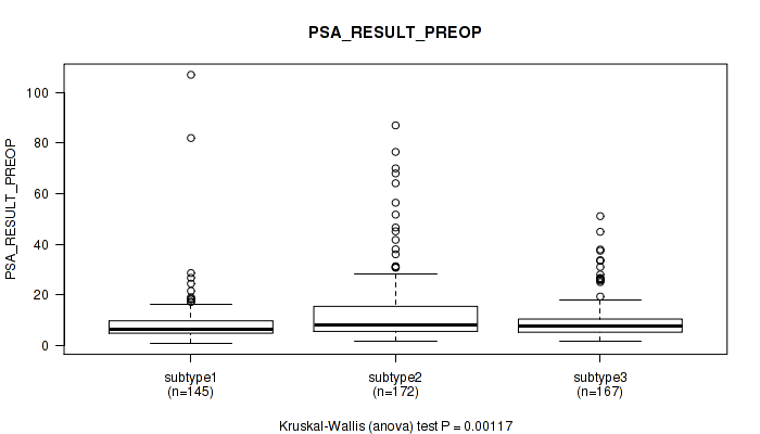
P value = 0.00117 (Kruskal-Wallis (anova)), Q value = 0.0031
Table S43. Clustering Approach #3: 'RNAseq CNMF subtypes' versus Clinical Feature #12: 'PSA_RESULT_PREOP'
| nPatients | Mean (Std.Dev) | |
|---|---|---|
| ALL | 484 | 10.9 (11.7) |
| subtype1 | 145 | 8.9 (11.3) |
| subtype2 | 172 | 13.6 (14.4) |
| subtype3 | 167 | 9.7 (8.0) |
Figure S40. Get High-res Image Clustering Approach #3: 'RNAseq CNMF subtypes' versus Clinical Feature #12: 'PSA_RESULT_PREOP'
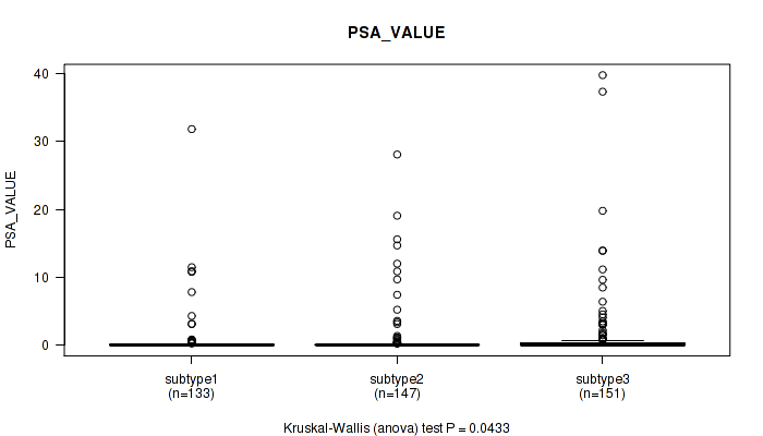
P value = 0.0433 (Kruskal-Wallis (anova)), Q value = 0.072
Table S44. Clustering Approach #3: 'RNAseq CNMF subtypes' versus Clinical Feature #13: 'PSA_VALUE'
| nPatients | Mean (Std.Dev) | |
|---|---|---|
| ALL | 431 | 1.1 (4.1) |
| subtype1 | 133 | 0.7 (3.3) |
| subtype2 | 147 | 1.0 (3.6) |
| subtype3 | 151 | 1.4 (5.1) |
Figure S41. Get High-res Image Clustering Approach #3: 'RNAseq CNMF subtypes' versus Clinical Feature #13: 'PSA_VALUE'
P value = 0.337 (Fisher's exact test), Q value = 0.43
Table S45. Clustering Approach #3: 'RNAseq CNMF subtypes' versus Clinical Feature #14: 'RACE'
| nPatients | ASIAN | BLACK OR AFRICAN AMERICAN | WHITE |
|---|---|---|---|
| ALL | 2 | 7 | 147 |
| subtype1 | 2 | 1 | 51 |
| subtype2 | 0 | 3 | 40 |
| subtype3 | 0 | 3 | 56 |
Figure S42. Get High-res Image Clustering Approach #3: 'RNAseq CNMF subtypes' versus Clinical Feature #14: 'RACE'
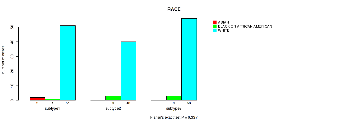
Table S46. Description of clustering approach #4: 'RNAseq cHierClus subtypes'
| Cluster Labels | 1 | 2 | 3 |
|---|---|---|---|
| Number of samples | 173 | 203 | 111 |
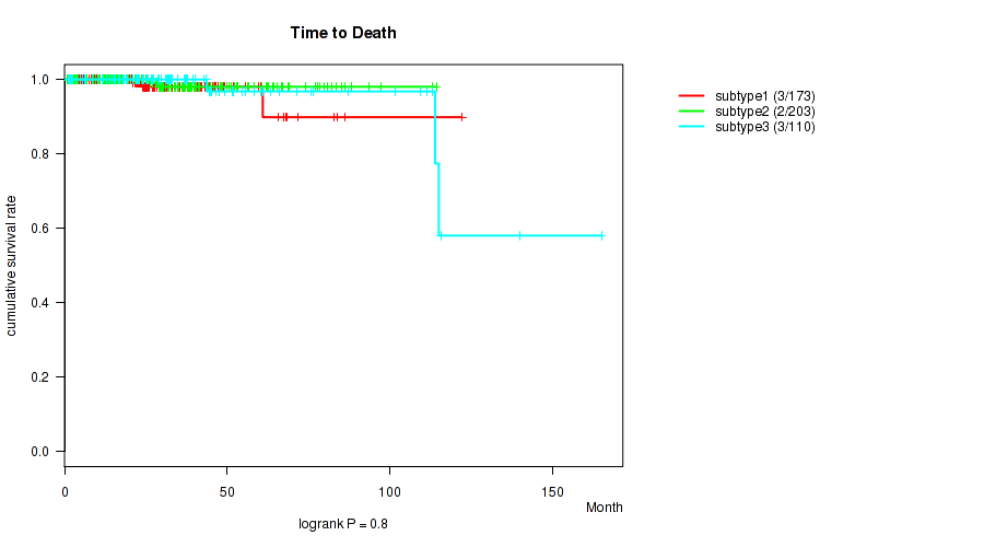
P value = 0.8 (logrank test), Q value = 0.83
Table S47. Clustering Approach #4: 'RNAseq cHierClus subtypes' versus Clinical Feature #1: 'Time to Death'
| nPatients | nDeath | Duration Range (Median), Month | |
|---|---|---|---|
| ALL | 486 | 8 | 0.7 - 165.2 (26.5) |
| subtype1 | 173 | 3 | 0.7 - 122.2 (25.1) |
| subtype2 | 203 | 2 | 0.8 - 114.4 (27.9) |
| subtype3 | 110 | 3 | 1.0 - 165.2 (26.2) |
Figure S43. Get High-res Image Clustering Approach #4: 'RNAseq cHierClus subtypes' versus Clinical Feature #1: 'Time to Death'
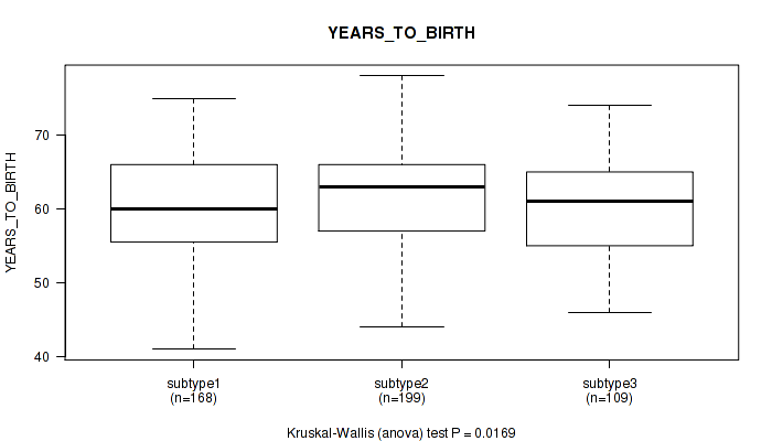
P value = 0.0169 (Kruskal-Wallis (anova)), Q value = 0.034
Table S48. Clustering Approach #4: 'RNAseq cHierClus subtypes' versus Clinical Feature #2: 'YEARS_TO_BIRTH'
| nPatients | Mean (Std.Dev) | |
|---|---|---|
| ALL | 476 | 60.9 (6.8) |
| subtype1 | 168 | 60.1 (6.8) |
| subtype2 | 199 | 62.1 (6.8) |
| subtype3 | 109 | 60.1 (6.5) |
Figure S44. Get High-res Image Clustering Approach #4: 'RNAseq cHierClus subtypes' versus Clinical Feature #2: 'YEARS_TO_BIRTH'
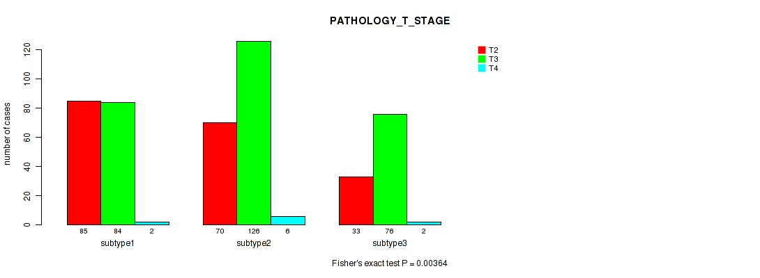
P value = 0.00364 (Fisher's exact test), Q value = 0.0087
Table S49. Clustering Approach #4: 'RNAseq cHierClus subtypes' versus Clinical Feature #3: 'PATHOLOGY_T_STAGE'
| nPatients | T2 | T3 | T4 |
|---|---|---|---|
| ALL | 188 | 286 | 10 |
| subtype1 | 85 | 84 | 2 |
| subtype2 | 70 | 126 | 6 |
| subtype3 | 33 | 76 | 2 |
Figure S45. Get High-res Image Clustering Approach #4: 'RNAseq cHierClus subtypes' versus Clinical Feature #3: 'PATHOLOGY_T_STAGE'
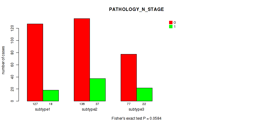
P value = 0.0584 (Fisher's exact test), Q value = 0.096
Table S50. Clustering Approach #4: 'RNAseq cHierClus subtypes' versus Clinical Feature #4: 'PATHOLOGY_N_STAGE'
| nPatients | 0 | 1 |
|---|---|---|
| ALL | 340 | 77 |
| subtype1 | 127 | 18 |
| subtype2 | 136 | 37 |
| subtype3 | 77 | 22 |
Figure S46. Get High-res Image Clustering Approach #4: 'RNAseq cHierClus subtypes' versus Clinical Feature #4: 'PATHOLOGY_N_STAGE'
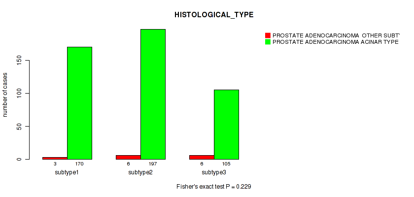
P value = 0.229 (Fisher's exact test), Q value = 0.31
Table S51. Clustering Approach #4: 'RNAseq cHierClus subtypes' versus Clinical Feature #5: 'HISTOLOGICAL_TYPE'
| nPatients | PROSTATE ADENOCARCINOMA OTHER SUBTYPE | PROSTATE ADENOCARCINOMA ACINAR TYPE |
|---|---|---|
| ALL | 15 | 472 |
| subtype1 | 3 | 170 |
| subtype2 | 6 | 197 |
| subtype3 | 6 | 105 |
Figure S47. Get High-res Image Clustering Approach #4: 'RNAseq cHierClus subtypes' versus Clinical Feature #5: 'HISTOLOGICAL_TYPE'
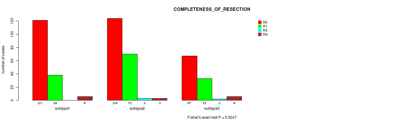
P value = 0.0247 (Fisher's exact test), Q value = 0.048
Table S52. Clustering Approach #4: 'RNAseq cHierClus subtypes' versus Clinical Feature #6: 'COMPLETENESS_OF_RESECTION'
| nPatients | R0 | R1 | R2 | RX |
|---|---|---|---|---|
| ALL | 312 | 141 | 5 | 15 |
| subtype1 | 121 | 38 | 0 | 6 |
| subtype2 | 124 | 70 | 3 | 3 |
| subtype3 | 67 | 33 | 2 | 6 |
Figure S48. Get High-res Image Clustering Approach #4: 'RNAseq cHierClus subtypes' versus Clinical Feature #6: 'COMPLETENESS_OF_RESECTION'
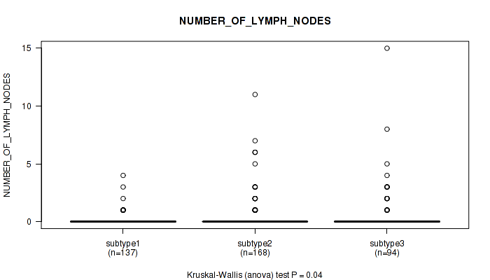
P value = 0.04 (Kruskal-Wallis (anova)), Q value = 0.069
Table S53. Clustering Approach #4: 'RNAseq cHierClus subtypes' versus Clinical Feature #7: 'NUMBER_OF_LYMPH_NODES'
| nPatients | Mean (Std.Dev) | |
|---|---|---|
| ALL | 399 | 0.4 (1.4) |
| subtype1 | 137 | 0.2 (0.5) |
| subtype2 | 168 | 0.5 (1.4) |
| subtype3 | 94 | 0.7 (2.0) |
Figure S49. Get High-res Image Clustering Approach #4: 'RNAseq cHierClus subtypes' versus Clinical Feature #7: 'NUMBER_OF_LYMPH_NODES'
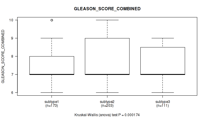
P value = 0.000174 (Kruskal-Wallis (anova)), Q value = 0.00061
Table S54. Clustering Approach #4: 'RNAseq cHierClus subtypes' versus Clinical Feature #8: 'GLEASON_SCORE_COMBINED'
| nPatients | Mean (Std.Dev) | |
|---|---|---|
| ALL | 487 | 7.6 (1.0) |
| subtype1 | 173 | 7.3 (0.9) |
| subtype2 | 203 | 7.8 (1.1) |
| subtype3 | 111 | 7.6 (1.0) |
Figure S50. Get High-res Image Clustering Approach #4: 'RNAseq cHierClus subtypes' versus Clinical Feature #8: 'GLEASON_SCORE_COMBINED'
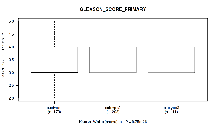
P value = 8.75e-06 (Kruskal-Wallis (anova)), Q value = 5.8e-05
Table S55. Clustering Approach #4: 'RNAseq cHierClus subtypes' versus Clinical Feature #9: 'GLEASON_SCORE_PRIMARY'
| nPatients | Mean (Std.Dev) | |
|---|---|---|
| ALL | 487 | 3.7 (0.7) |
| subtype1 | 173 | 3.5 (0.7) |
| subtype2 | 203 | 3.9 (0.7) |
| subtype3 | 111 | 3.7 (0.6) |
Figure S51. Get High-res Image Clustering Approach #4: 'RNAseq cHierClus subtypes' versus Clinical Feature #9: 'GLEASON_SCORE_PRIMARY'
P value = 0.25 (Kruskal-Wallis (anova)), Q value = 0.34
Table S56. Clustering Approach #4: 'RNAseq cHierClus subtypes' versus Clinical Feature #10: 'GLEASON_SCORE_SECONDARY'
| nPatients | Mean (Std.Dev) | |
|---|---|---|
| ALL | 487 | 3.9 (0.7) |
| subtype1 | 173 | 3.8 (0.6) |
| subtype2 | 203 | 3.9 (0.7) |
| subtype3 | 111 | 3.9 (0.7) |
Figure S52. Get High-res Image Clustering Approach #4: 'RNAseq cHierClus subtypes' versus Clinical Feature #10: 'GLEASON_SCORE_SECONDARY'

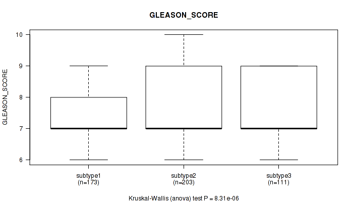
P value = 8.31e-06 (Kruskal-Wallis (anova)), Q value = 5.8e-05
Table S57. Clustering Approach #4: 'RNAseq cHierClus subtypes' versus Clinical Feature #11: 'GLEASON_SCORE'
| nPatients | Mean (Std.Dev) | |
|---|---|---|
| ALL | 487 | 7.6 (1.0) |
| subtype1 | 173 | 7.3 (0.9) |
| subtype2 | 203 | 7.8 (1.1) |
| subtype3 | 111 | 7.7 (1.0) |
Figure S53. Get High-res Image Clustering Approach #4: 'RNAseq cHierClus subtypes' versus Clinical Feature #11: 'GLEASON_SCORE'
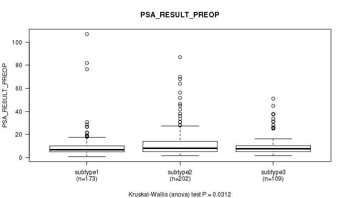
P value = 0.0312 (Kruskal-Wallis (anova)), Q value = 0.059
Table S58. Clustering Approach #4: 'RNAseq cHierClus subtypes' versus Clinical Feature #12: 'PSA_RESULT_PREOP'
| nPatients | Mean (Std.Dev) | |
|---|---|---|
| ALL | 484 | 10.9 (11.7) |
| subtype1 | 173 | 9.5 (11.8) |
| subtype2 | 202 | 12.3 (12.8) |
| subtype3 | 109 | 10.3 (9.0) |
Figure S54. Get High-res Image Clustering Approach #4: 'RNAseq cHierClus subtypes' versus Clinical Feature #12: 'PSA_RESULT_PREOP'
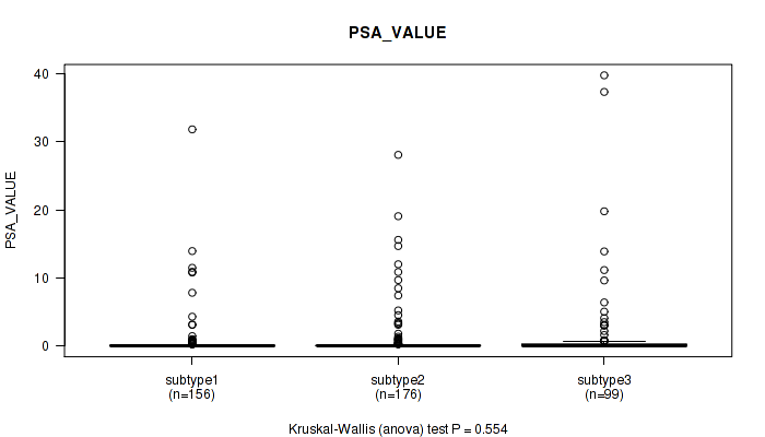
P value = 0.554 (Kruskal-Wallis (anova)), Q value = 0.65
Table S59. Clustering Approach #4: 'RNAseq cHierClus subtypes' versus Clinical Feature #13: 'PSA_VALUE'
| nPatients | Mean (Std.Dev) | |
|---|---|---|
| ALL | 431 | 1.1 (4.1) |
| subtype1 | 156 | 0.8 (3.2) |
| subtype2 | 176 | 1.0 (3.4) |
| subtype3 | 99 | 1.8 (6.1) |
Figure S55. Get High-res Image Clustering Approach #4: 'RNAseq cHierClus subtypes' versus Clinical Feature #13: 'PSA_VALUE'
P value = 0.0226 (Fisher's exact test), Q value = 0.045
Table S60. Clustering Approach #4: 'RNAseq cHierClus subtypes' versus Clinical Feature #14: 'RACE'
| nPatients | ASIAN | BLACK OR AFRICAN AMERICAN | WHITE |
|---|---|---|---|
| ALL | 2 | 7 | 147 |
| subtype1 | 2 | 0 | 65 |
| subtype2 | 0 | 5 | 46 |
| subtype3 | 0 | 2 | 36 |
Figure S56. Get High-res Image Clustering Approach #4: 'RNAseq cHierClus subtypes' versus Clinical Feature #14: 'RACE'
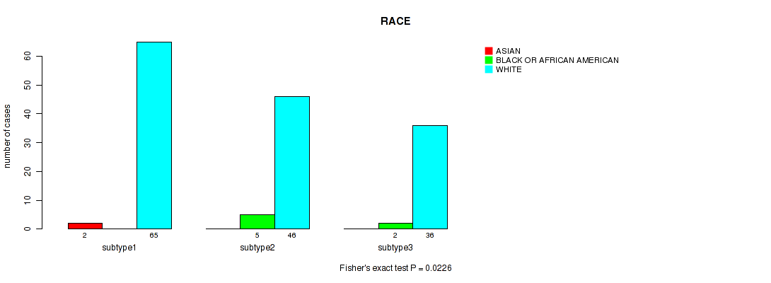
Table S61. Description of clustering approach #5: 'MIRSEQ CNMF'
| Cluster Labels | 1 | 2 | 3 |
|---|---|---|---|
| Number of samples | 157 | 145 | 182 |
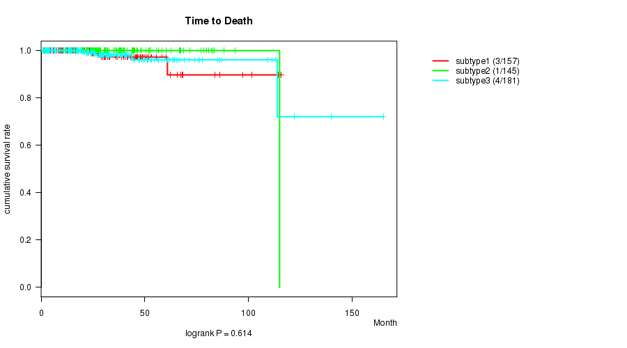
P value = 0.614 (logrank test), Q value = 0.7
Table S62. Clustering Approach #5: 'MIRSEQ CNMF' versus Clinical Feature #1: 'Time to Death'
| nPatients | nDeath | Duration Range (Median), Month | |
|---|---|---|---|
| ALL | 483 | 8 | 0.7 - 165.2 (26.3) |
| subtype1 | 157 | 3 | 1.0 - 115.9 (23.9) |
| subtype2 | 145 | 1 | 0.7 - 115.1 (26.7) |
| subtype3 | 181 | 4 | 0.8 - 165.2 (28.9) |
Figure S57. Get High-res Image Clustering Approach #5: 'MIRSEQ CNMF' versus Clinical Feature #1: 'Time to Death'
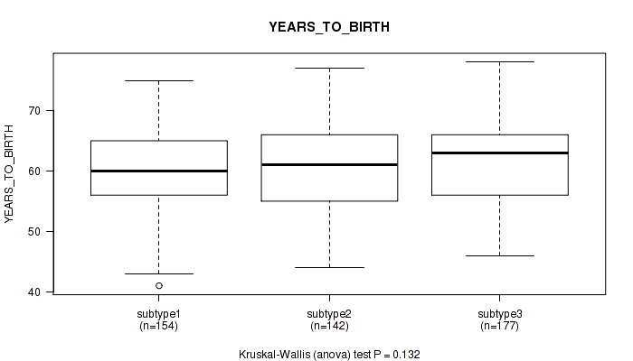
P value = 0.132 (Kruskal-Wallis (anova)), Q value = 0.2
Table S63. Clustering Approach #5: 'MIRSEQ CNMF' versus Clinical Feature #2: 'YEARS_TO_BIRTH'
| nPatients | Mean (Std.Dev) | |
|---|---|---|
| ALL | 473 | 60.9 (6.8) |
| subtype1 | 154 | 60.2 (6.5) |
| subtype2 | 142 | 60.7 (7.3) |
| subtype3 | 177 | 61.8 (6.7) |
Figure S58. Get High-res Image Clustering Approach #5: 'MIRSEQ CNMF' versus Clinical Feature #2: 'YEARS_TO_BIRTH'
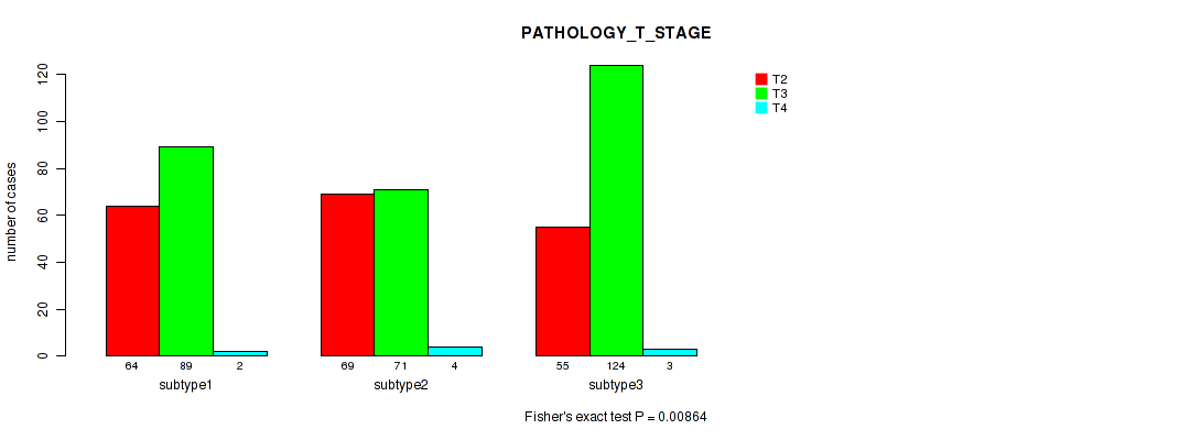
P value = 0.00864 (Fisher's exact test), Q value = 0.019
Table S64. Clustering Approach #5: 'MIRSEQ CNMF' versus Clinical Feature #3: 'PATHOLOGY_T_STAGE'
| nPatients | T2 | T3 | T4 |
|---|---|---|---|
| ALL | 188 | 284 | 9 |
| subtype1 | 64 | 89 | 2 |
| subtype2 | 69 | 71 | 4 |
| subtype3 | 55 | 124 | 3 |
Figure S59. Get High-res Image Clustering Approach #5: 'MIRSEQ CNMF' versus Clinical Feature #3: 'PATHOLOGY_T_STAGE'
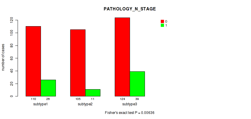
P value = 0.00636 (Fisher's exact test), Q value = 0.014
Table S65. Clustering Approach #5: 'MIRSEQ CNMF' versus Clinical Feature #4: 'PATHOLOGY_N_STAGE'
| nPatients | 0 | 1 |
|---|---|---|
| ALL | 339 | 76 |
| subtype1 | 110 | 26 |
| subtype2 | 105 | 11 |
| subtype3 | 124 | 39 |
Figure S60. Get High-res Image Clustering Approach #5: 'MIRSEQ CNMF' versus Clinical Feature #4: 'PATHOLOGY_N_STAGE'
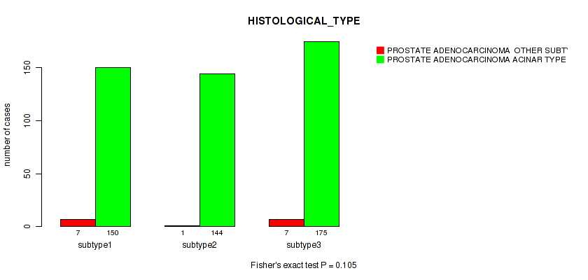
P value = 0.105 (Fisher's exact test), Q value = 0.16
Table S66. Clustering Approach #5: 'MIRSEQ CNMF' versus Clinical Feature #5: 'HISTOLOGICAL_TYPE'
| nPatients | PROSTATE ADENOCARCINOMA OTHER SUBTYPE | PROSTATE ADENOCARCINOMA ACINAR TYPE |
|---|---|---|
| ALL | 15 | 469 |
| subtype1 | 7 | 150 |
| subtype2 | 1 | 144 |
| subtype3 | 7 | 175 |
Figure S61. Get High-res Image Clustering Approach #5: 'MIRSEQ CNMF' versus Clinical Feature #5: 'HISTOLOGICAL_TYPE'
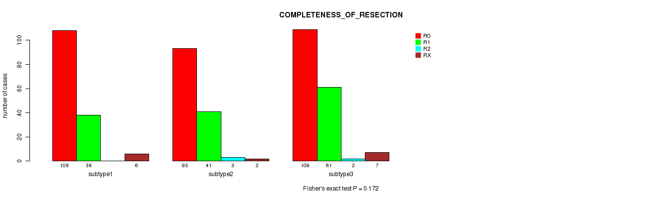
P value = 0.172 (Fisher's exact test), Q value = 0.24
Table S67. Clustering Approach #5: 'MIRSEQ CNMF' versus Clinical Feature #6: 'COMPLETENESS_OF_RESECTION'
| nPatients | R0 | R1 | R2 | RX |
|---|---|---|---|---|
| ALL | 310 | 140 | 5 | 15 |
| subtype1 | 108 | 38 | 0 | 6 |
| subtype2 | 93 | 41 | 3 | 2 |
| subtype3 | 109 | 61 | 2 | 7 |
Figure S62. Get High-res Image Clustering Approach #5: 'MIRSEQ CNMF' versus Clinical Feature #6: 'COMPLETENESS_OF_RESECTION'
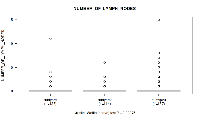
P value = 0.00375 (Kruskal-Wallis (anova)), Q value = 0.0088
Table S68. Clustering Approach #5: 'MIRSEQ CNMF' versus Clinical Feature #7: 'NUMBER_OF_LYMPH_NODES'
| nPatients | Mean (Std.Dev) | |
|---|---|---|
| ALL | 397 | 0.4 (1.4) |
| subtype1 | 126 | 0.3 (1.1) |
| subtype2 | 114 | 0.2 (0.7) |
| subtype3 | 157 | 0.7 (1.8) |
Figure S63. Get High-res Image Clustering Approach #5: 'MIRSEQ CNMF' versus Clinical Feature #7: 'NUMBER_OF_LYMPH_NODES'
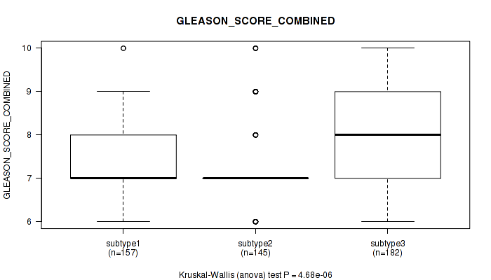
P value = 4.68e-06 (Kruskal-Wallis (anova)), Q value = 3.7e-05
Table S69. Clustering Approach #5: 'MIRSEQ CNMF' versus Clinical Feature #8: 'GLEASON_SCORE_COMBINED'
| nPatients | Mean (Std.Dev) | |
|---|---|---|
| ALL | 484 | 7.6 (1.0) |
| subtype1 | 157 | 7.5 (1.0) |
| subtype2 | 145 | 7.3 (1.0) |
| subtype3 | 182 | 7.8 (1.0) |
Figure S64. Get High-res Image Clustering Approach #5: 'MIRSEQ CNMF' versus Clinical Feature #8: 'GLEASON_SCORE_COMBINED'
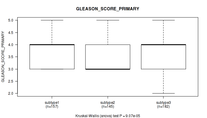
P value = 9.07e-05 (Kruskal-Wallis (anova)), Q value = 0.00035
Table S70. Clustering Approach #5: 'MIRSEQ CNMF' versus Clinical Feature #9: 'GLEASON_SCORE_PRIMARY'
| nPatients | Mean (Std.Dev) | |
|---|---|---|
| ALL | 484 | 3.7 (0.7) |
| subtype1 | 157 | 3.6 (0.6) |
| subtype2 | 145 | 3.6 (0.7) |
| subtype3 | 182 | 3.8 (0.7) |
Figure S65. Get High-res Image Clustering Approach #5: 'MIRSEQ CNMF' versus Clinical Feature #9: 'GLEASON_SCORE_PRIMARY'
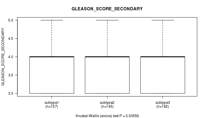
P value = 0.00559 (Kruskal-Wallis (anova)), Q value = 0.013
Table S71. Clustering Approach #5: 'MIRSEQ CNMF' versus Clinical Feature #10: 'GLEASON_SCORE_SECONDARY'
| nPatients | Mean (Std.Dev) | |
|---|---|---|
| ALL | 484 | 3.9 (0.7) |
| subtype1 | 157 | 3.9 (0.7) |
| subtype2 | 145 | 3.7 (0.7) |
| subtype3 | 182 | 3.9 (0.7) |
Figure S66. Get High-res Image Clustering Approach #5: 'MIRSEQ CNMF' versus Clinical Feature #10: 'GLEASON_SCORE_SECONDARY'
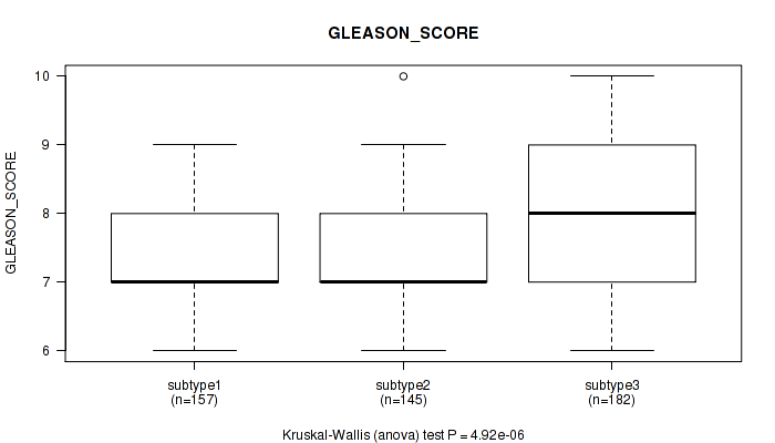
P value = 4.92e-06 (Kruskal-Wallis (anova)), Q value = 3.7e-05
Table S72. Clustering Approach #5: 'MIRSEQ CNMF' versus Clinical Feature #11: 'GLEASON_SCORE'
| nPatients | Mean (Std.Dev) | |
|---|---|---|
| ALL | 484 | 7.6 (1.0) |
| subtype1 | 157 | 7.5 (0.9) |
| subtype2 | 145 | 7.3 (1.0) |
| subtype3 | 182 | 7.9 (1.0) |
Figure S67. Get High-res Image Clustering Approach #5: 'MIRSEQ CNMF' versus Clinical Feature #11: 'GLEASON_SCORE'
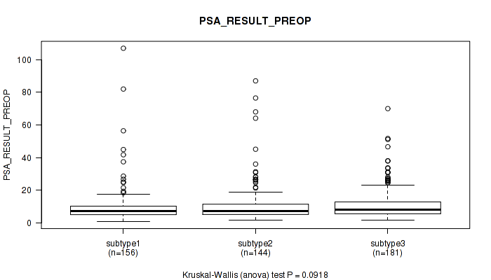
P value = 0.0918 (Kruskal-Wallis (anova)), Q value = 0.14
Table S73. Clustering Approach #5: 'MIRSEQ CNMF' versus Clinical Feature #12: 'PSA_RESULT_PREOP'
| nPatients | Mean (Std.Dev) | |
|---|---|---|
| ALL | 481 | 10.9 (11.7) |
| subtype1 | 156 | 10.0 (12.4) |
| subtype2 | 144 | 11.3 (13.0) |
| subtype3 | 181 | 11.2 (10.0) |
Figure S68. Get High-res Image Clustering Approach #5: 'MIRSEQ CNMF' versus Clinical Feature #12: 'PSA_RESULT_PREOP'
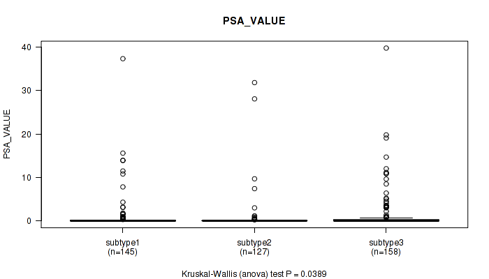
P value = 0.0389 (Kruskal-Wallis (anova)), Q value = 0.069
Table S74. Clustering Approach #5: 'MIRSEQ CNMF' versus Clinical Feature #13: 'PSA_VALUE'
| nPatients | Mean (Std.Dev) | |
|---|---|---|
| ALL | 430 | 1.1 (4.1) |
| subtype1 | 145 | 1.0 (3.9) |
| subtype2 | 127 | 0.7 (3.9) |
| subtype3 | 158 | 1.4 (4.5) |
Figure S69. Get High-res Image Clustering Approach #5: 'MIRSEQ CNMF' versus Clinical Feature #13: 'PSA_VALUE'
P value = 0.215 (Fisher's exact test), Q value = 0.3
Table S75. Clustering Approach #5: 'MIRSEQ CNMF' versus Clinical Feature #14: 'RACE'
| nPatients | ASIAN | BLACK OR AFRICAN AMERICAN | WHITE |
|---|---|---|---|
| ALL | 2 | 7 | 146 |
| subtype1 | 1 | 0 | 39 |
| subtype2 | 1 | 3 | 69 |
| subtype3 | 0 | 4 | 38 |
Figure S70. Get High-res Image Clustering Approach #5: 'MIRSEQ CNMF' versus Clinical Feature #14: 'RACE'
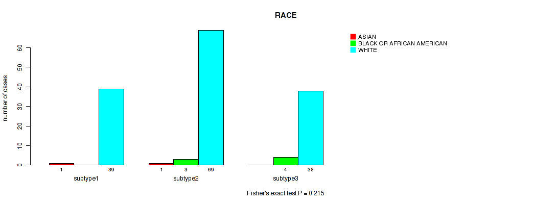
Table S76. Description of clustering approach #6: 'MIRSEQ CHIERARCHICAL'
| Cluster Labels | 1 | 2 | 3 | 4 | 5 |
|---|---|---|---|---|---|
| Number of samples | 147 | 97 | 59 | 125 | 56 |
P value = 0.823 (logrank test), Q value = 0.85
Table S77. Clustering Approach #6: 'MIRSEQ CHIERARCHICAL' versus Clinical Feature #1: 'Time to Death'
| nPatients | nDeath | Duration Range (Median), Month | |
|---|---|---|---|
| ALL | 483 | 8 | 0.7 - 165.2 (26.3) |
| subtype1 | 147 | 2 | 1.0 - 115.9 (25.5) |
| subtype2 | 97 | 2 | 2.2 - 115.1 (28.2) |
| subtype3 | 59 | 2 | 1.0 - 140.2 (24.0) |
| subtype4 | 125 | 1 | 0.8 - 165.2 (28.2) |
| subtype5 | 55 | 1 | 0.7 - 111.4 (25.7) |
Figure S71. Get High-res Image Clustering Approach #6: 'MIRSEQ CHIERARCHICAL' versus Clinical Feature #1: 'Time to Death'
P value = 0.0401 (Kruskal-Wallis (anova)), Q value = 0.069
Table S78. Clustering Approach #6: 'MIRSEQ CHIERARCHICAL' versus Clinical Feature #2: 'YEARS_TO_BIRTH'
| nPatients | Mean (Std.Dev) | |
|---|---|---|
| ALL | 473 | 60.9 (6.8) |
| subtype1 | 144 | 60.5 (6.6) |
| subtype2 | 94 | 60.6 (6.7) |
| subtype3 | 59 | 59.6 (6.4) |
| subtype4 | 122 | 62.6 (6.8) |
| subtype5 | 54 | 60.4 (7.6) |
Figure S72. Get High-res Image Clustering Approach #6: 'MIRSEQ CHIERARCHICAL' versus Clinical Feature #2: 'YEARS_TO_BIRTH'
P value = 2e-05 (Fisher's exact test), Q value = 9.3e-05
Table S79. Clustering Approach #6: 'MIRSEQ CHIERARCHICAL' versus Clinical Feature #3: 'PATHOLOGY_T_STAGE'
| nPatients | T2 | T3 | T4 |
|---|---|---|---|
| ALL | 188 | 284 | 9 |
| subtype1 | 65 | 80 | 0 |
| subtype2 | 45 | 47 | 4 |
| subtype3 | 21 | 37 | 1 |
| subtype4 | 27 | 94 | 4 |
| subtype5 | 30 | 26 | 0 |
Figure S73. Get High-res Image Clustering Approach #6: 'MIRSEQ CHIERARCHICAL' versus Clinical Feature #3: 'PATHOLOGY_T_STAGE'
P value = 0.00025 (Fisher's exact test), Q value = 0.00082
Table S80. Clustering Approach #6: 'MIRSEQ CHIERARCHICAL' versus Clinical Feature #4: 'PATHOLOGY_N_STAGE'
| nPatients | 0 | 1 |
|---|---|---|
| ALL | 339 | 76 |
| subtype1 | 110 | 18 |
| subtype2 | 70 | 8 |
| subtype3 | 40 | 12 |
| subtype4 | 78 | 35 |
| subtype5 | 41 | 3 |
Figure S74. Get High-res Image Clustering Approach #6: 'MIRSEQ CHIERARCHICAL' versus Clinical Feature #4: 'PATHOLOGY_N_STAGE'
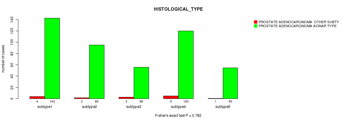
P value = 0.782 (Fisher's exact test), Q value = 0.83
Table S81. Clustering Approach #6: 'MIRSEQ CHIERARCHICAL' versus Clinical Feature #5: 'HISTOLOGICAL_TYPE'
| nPatients | PROSTATE ADENOCARCINOMA OTHER SUBTYPE | PROSTATE ADENOCARCINOMA ACINAR TYPE |
|---|---|---|
| ALL | 15 | 469 |
| subtype1 | 4 | 143 |
| subtype2 | 2 | 95 |
| subtype3 | 3 | 56 |
| subtype4 | 5 | 120 |
| subtype5 | 1 | 55 |
Figure S75. Get High-res Image Clustering Approach #6: 'MIRSEQ CHIERARCHICAL' versus Clinical Feature #5: 'HISTOLOGICAL_TYPE'
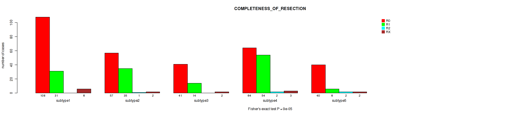
P value = 9e-05 (Fisher's exact test), Q value = 0.00035
Table S82. Clustering Approach #6: 'MIRSEQ CHIERARCHICAL' versus Clinical Feature #6: 'COMPLETENESS_OF_RESECTION'
| nPatients | R0 | R1 | R2 | RX |
|---|---|---|---|---|
| ALL | 310 | 140 | 5 | 15 |
| subtype1 | 108 | 31 | 0 | 6 |
| subtype2 | 57 | 35 | 1 | 2 |
| subtype3 | 41 | 14 | 0 | 2 |
| subtype4 | 64 | 54 | 2 | 3 |
| subtype5 | 40 | 6 | 2 | 2 |
Figure S76. Get High-res Image Clustering Approach #6: 'MIRSEQ CHIERARCHICAL' versus Clinical Feature #6: 'COMPLETENESS_OF_RESECTION'
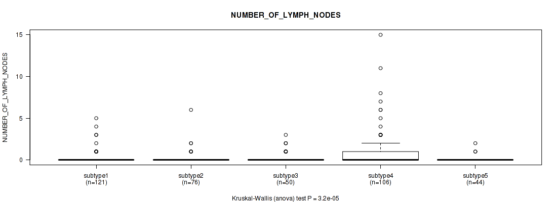
P value = 3.2e-05 (Kruskal-Wallis (anova)), Q value = 0.00014
Table S83. Clustering Approach #6: 'MIRSEQ CHIERARCHICAL' versus Clinical Feature #7: 'NUMBER_OF_LYMPH_NODES'
| nPatients | Mean (Std.Dev) | |
|---|---|---|
| ALL | 397 | 0.4 (1.4) |
| subtype1 | 121 | 0.2 (0.8) |
| subtype2 | 76 | 0.2 (0.8) |
| subtype3 | 50 | 0.3 (0.7) |
| subtype4 | 106 | 1.0 (2.3) |
| subtype5 | 44 | 0.1 (0.4) |
Figure S77. Get High-res Image Clustering Approach #6: 'MIRSEQ CHIERARCHICAL' versus Clinical Feature #7: 'NUMBER_OF_LYMPH_NODES'
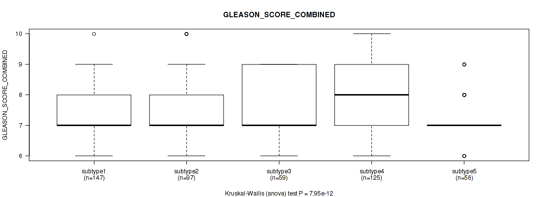
P value = 7.95e-12 (Kruskal-Wallis (anova)), Q value = 2.2e-10
Table S84. Clustering Approach #6: 'MIRSEQ CHIERARCHICAL' versus Clinical Feature #8: 'GLEASON_SCORE_COMBINED'
| nPatients | Mean (Std.Dev) | |
|---|---|---|
| ALL | 484 | 7.6 (1.0) |
| subtype1 | 147 | 7.4 (0.9) |
| subtype2 | 97 | 7.3 (1.1) |
| subtype3 | 59 | 7.6 (1.0) |
| subtype4 | 125 | 8.1 (1.0) |
| subtype5 | 56 | 7.2 (0.7) |
Figure S78. Get High-res Image Clustering Approach #6: 'MIRSEQ CHIERARCHICAL' versus Clinical Feature #8: 'GLEASON_SCORE_COMBINED'
P value = 1.07e-08 (Kruskal-Wallis (anova)), Q value = 1.3e-07
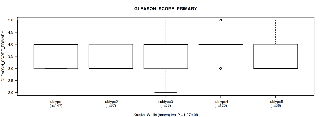
Table S85. Clustering Approach #6: 'MIRSEQ CHIERARCHICAL' versus Clinical Feature #9: 'GLEASON_SCORE_PRIMARY'
| nPatients | Mean (Std.Dev) | |
|---|---|---|
| ALL | 484 | 3.7 (0.7) |
| subtype1 | 147 | 3.6 (0.6) |
| subtype2 | 97 | 3.6 (0.7) |
| subtype3 | 59 | 3.7 (0.7) |
| subtype4 | 125 | 4.0 (0.7) |
| subtype5 | 56 | 3.5 (0.5) |
Figure S79. Get High-res Image Clustering Approach #6: 'MIRSEQ CHIERARCHICAL' versus Clinical Feature #9: 'GLEASON_SCORE_PRIMARY'
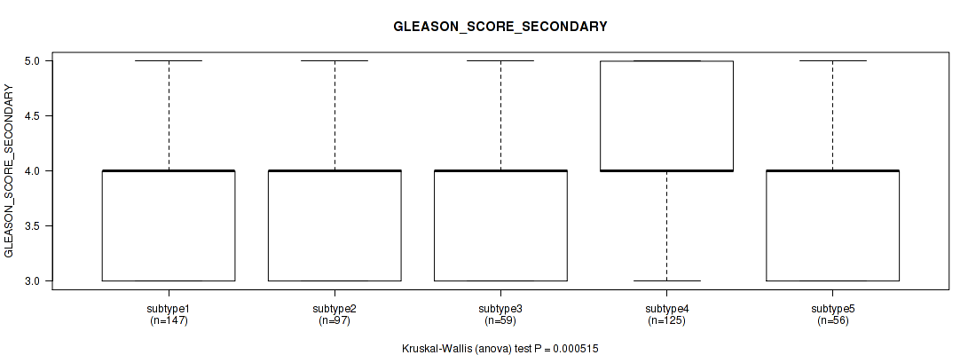
P value = 0.000515 (Kruskal-Wallis (anova)), Q value = 0.0015
Table S86. Clustering Approach #6: 'MIRSEQ CHIERARCHICAL' versus Clinical Feature #10: 'GLEASON_SCORE_SECONDARY'
| nPatients | Mean (Std.Dev) | |
|---|---|---|
| ALL | 484 | 3.9 (0.7) |
| subtype1 | 147 | 3.8 (0.7) |
| subtype2 | 97 | 3.7 (0.7) |
| subtype3 | 59 | 3.9 (0.7) |
| subtype4 | 125 | 4.1 (0.7) |
| subtype5 | 56 | 3.7 (0.6) |
Figure S80. Get High-res Image Clustering Approach #6: 'MIRSEQ CHIERARCHICAL' versus Clinical Feature #10: 'GLEASON_SCORE_SECONDARY'
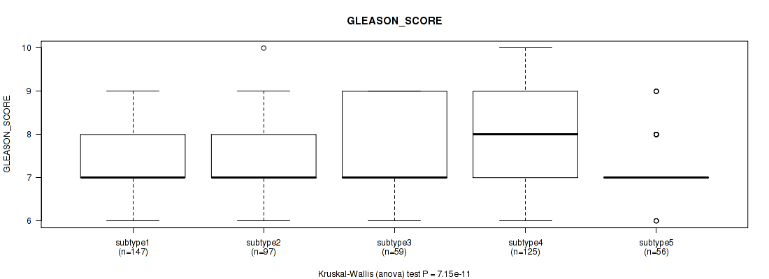
P value = 7.15e-11 (Kruskal-Wallis (anova)), Q value = 1.6e-09
Table S87. Clustering Approach #6: 'MIRSEQ CHIERARCHICAL' versus Clinical Feature #11: 'GLEASON_SCORE'
| nPatients | Mean (Std.Dev) | |
|---|---|---|
| ALL | 484 | 7.6 (1.0) |
| subtype1 | 147 | 7.4 (0.9) |
| subtype2 | 97 | 7.3 (1.1) |
| subtype3 | 59 | 7.6 (1.0) |
| subtype4 | 125 | 8.1 (1.0) |
| subtype5 | 56 | 7.2 (0.7) |
Figure S81. Get High-res Image Clustering Approach #6: 'MIRSEQ CHIERARCHICAL' versus Clinical Feature #11: 'GLEASON_SCORE'
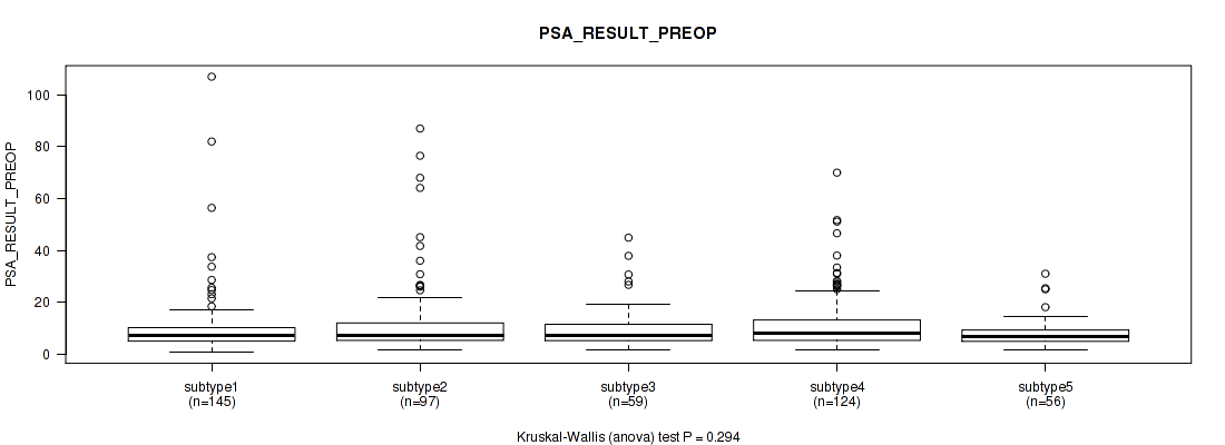
P value = 0.294 (Kruskal-Wallis (anova)), Q value = 0.38
Table S88. Clustering Approach #6: 'MIRSEQ CHIERARCHICAL' versus Clinical Feature #12: 'PSA_RESULT_PREOP'
| nPatients | Mean (Std.Dev) | |
|---|---|---|
| ALL | 481 | 10.9 (11.7) |
| subtype1 | 145 | 10.0 (12.3) |
| subtype2 | 97 | 12.8 (15.3) |
| subtype3 | 59 | 10.1 (8.5) |
| subtype4 | 124 | 11.8 (11.0) |
| subtype5 | 56 | 8.3 (5.7) |
Figure S82. Get High-res Image Clustering Approach #6: 'MIRSEQ CHIERARCHICAL' versus Clinical Feature #12: 'PSA_RESULT_PREOP'
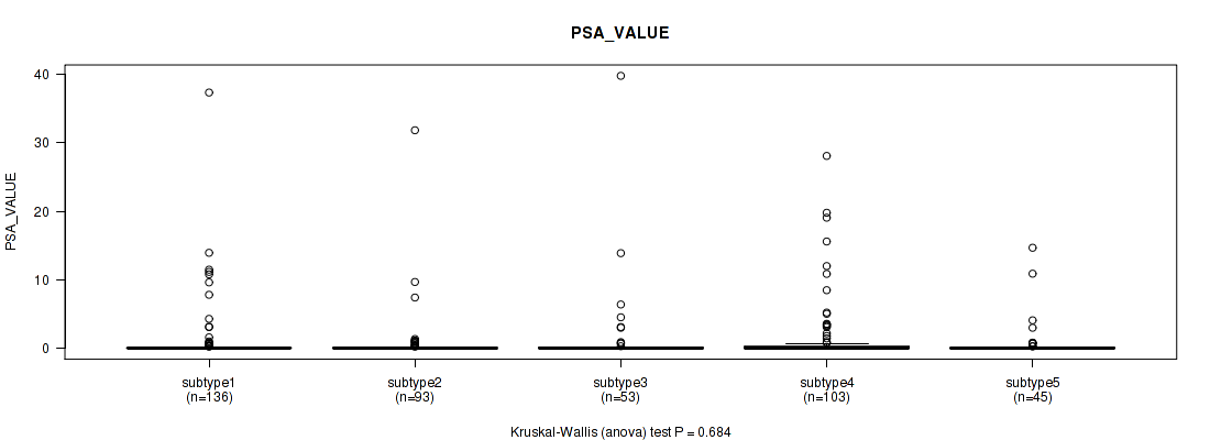
P value = 0.684 (Kruskal-Wallis (anova)), Q value = 0.76
Table S89. Clustering Approach #6: 'MIRSEQ CHIERARCHICAL' versus Clinical Feature #13: 'PSA_VALUE'
| nPatients | Mean (Std.Dev) | |
|---|---|---|
| ALL | 430 | 1.1 (4.1) |
| subtype1 | 136 | 0.9 (3.9) |
| subtype2 | 93 | 0.7 (3.5) |
| subtype3 | 53 | 1.4 (5.8) |
| subtype4 | 103 | 1.5 (4.4) |
| subtype5 | 45 | 0.9 (2.7) |
Figure S83. Get High-res Image Clustering Approach #6: 'MIRSEQ CHIERARCHICAL' versus Clinical Feature #13: 'PSA_VALUE'
P value = 0.708 (Fisher's exact test), Q value = 0.78
Table S90. Clustering Approach #6: 'MIRSEQ CHIERARCHICAL' versus Clinical Feature #14: 'RACE'
| nPatients | ASIAN | BLACK OR AFRICAN AMERICAN | WHITE |
|---|---|---|---|
| ALL | 2 | 7 | 146 |
| subtype1 | 1 | 1 | 51 |
| subtype2 | 0 | 3 | 30 |
| subtype3 | 0 | 0 | 18 |
| subtype4 | 0 | 0 | 9 |
| subtype5 | 1 | 3 | 38 |
Figure S84. Get High-res Image Clustering Approach #6: 'MIRSEQ CHIERARCHICAL' versus Clinical Feature #14: 'RACE'
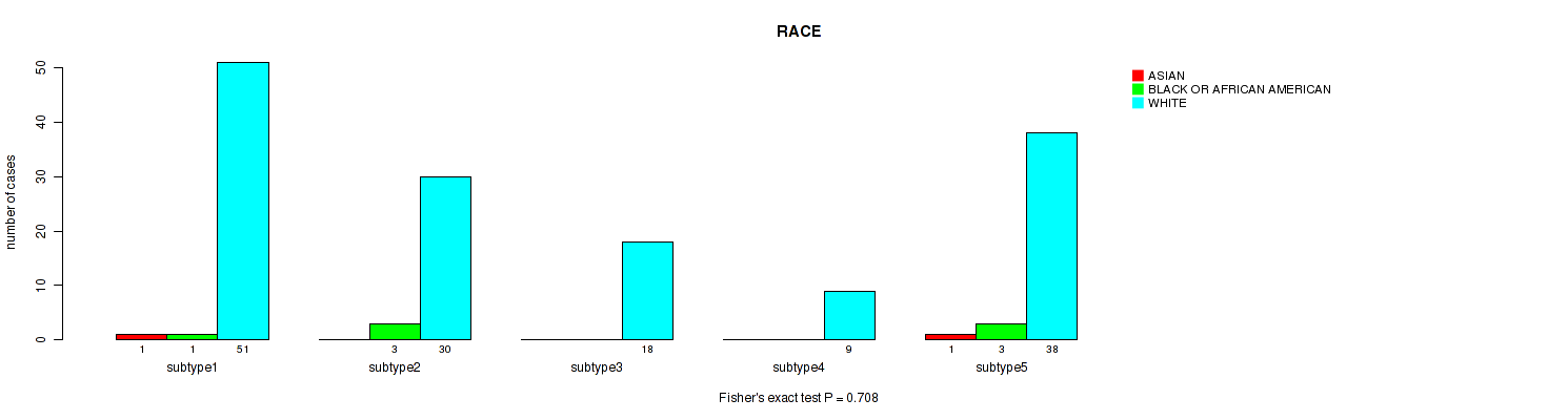
Table S91. Description of clustering approach #7: 'MIRseq Mature CNMF subtypes'
| Cluster Labels | 1 | 2 | 3 | 4 |
|---|---|---|---|---|
| Number of samples | 62 | 103 | 58 | 88 |
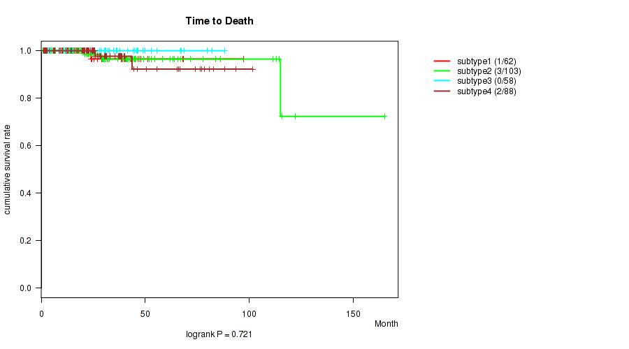
P value = 0.721 (logrank test), Q value = 0.78
Table S92. Clustering Approach #7: 'MIRseq Mature CNMF subtypes' versus Clinical Feature #1: 'Time to Death'
| nPatients | nDeath | Duration Range (Median), Month | |
|---|---|---|---|
| ALL | 311 | 6 | 0.8 - 165.2 (25.4) |
| subtype1 | 62 | 1 | 1.0 - 97.4 (22.0) |
| subtype2 | 103 | 3 | 0.8 - 165.2 (28.2) |
| subtype3 | 58 | 0 | 1.6 - 88.2 (28.4) |
| subtype4 | 88 | 2 | 1.1 - 101.8 (25.8) |
Figure S85. Get High-res Image Clustering Approach #7: 'MIRseq Mature CNMF subtypes' versus Clinical Feature #1: 'Time to Death'
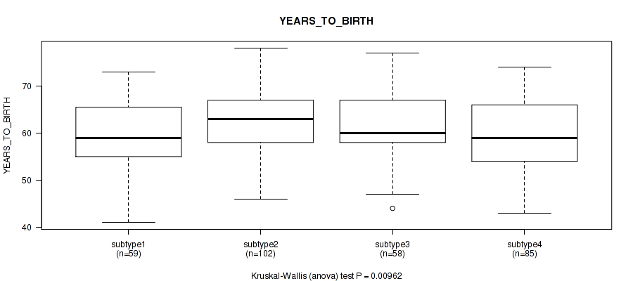
P value = 0.00962 (Kruskal-Wallis (anova)), Q value = 0.02
Table S93. Clustering Approach #7: 'MIRseq Mature CNMF subtypes' versus Clinical Feature #2: 'YEARS_TO_BIRTH'
| nPatients | Mean (Std.Dev) | |
|---|---|---|
| ALL | 304 | 60.9 (7.0) |
| subtype1 | 59 | 59.7 (7.4) |
| subtype2 | 102 | 62.7 (6.1) |
| subtype3 | 58 | 61.3 (6.8) |
| subtype4 | 85 | 59.3 (7.4) |
Figure S86. Get High-res Image Clustering Approach #7: 'MIRseq Mature CNMF subtypes' versus Clinical Feature #2: 'YEARS_TO_BIRTH'
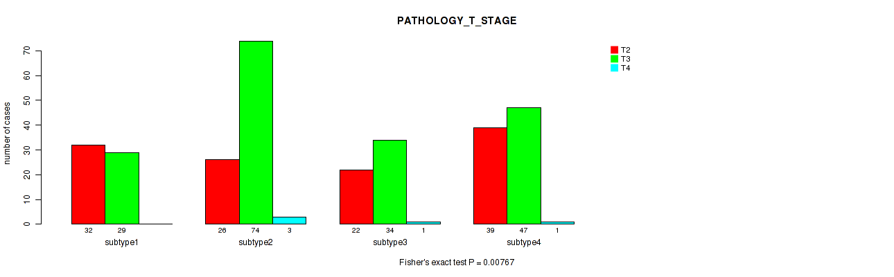
P value = 0.00767 (Fisher's exact test), Q value = 0.017
Table S94. Clustering Approach #7: 'MIRseq Mature CNMF subtypes' versus Clinical Feature #3: 'PATHOLOGY_T_STAGE'
| nPatients | T2 | T3 | T4 |
|---|---|---|---|
| ALL | 119 | 184 | 5 |
| subtype1 | 32 | 29 | 0 |
| subtype2 | 26 | 74 | 3 |
| subtype3 | 22 | 34 | 1 |
| subtype4 | 39 | 47 | 1 |
Figure S87. Get High-res Image Clustering Approach #7: 'MIRseq Mature CNMF subtypes' versus Clinical Feature #3: 'PATHOLOGY_T_STAGE'
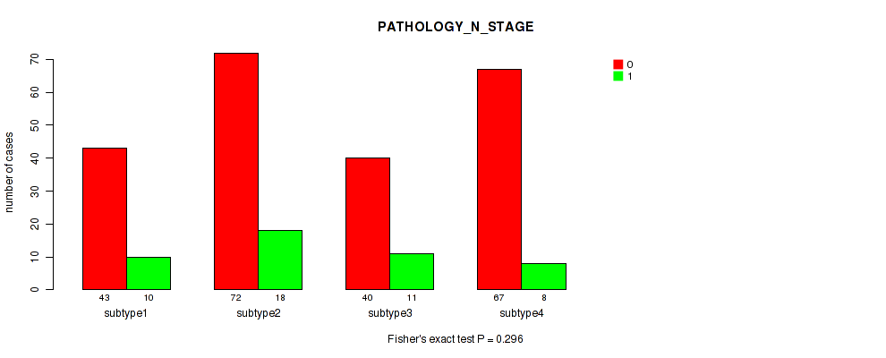
P value = 0.296 (Fisher's exact test), Q value = 0.38
Table S95. Clustering Approach #7: 'MIRseq Mature CNMF subtypes' versus Clinical Feature #4: 'PATHOLOGY_N_STAGE'
| nPatients | 0 | 1 |
|---|---|---|
| ALL | 222 | 47 |
| subtype1 | 43 | 10 |
| subtype2 | 72 | 18 |
| subtype3 | 40 | 11 |
| subtype4 | 67 | 8 |
Figure S88. Get High-res Image Clustering Approach #7: 'MIRseq Mature CNMF subtypes' versus Clinical Feature #4: 'PATHOLOGY_N_STAGE'
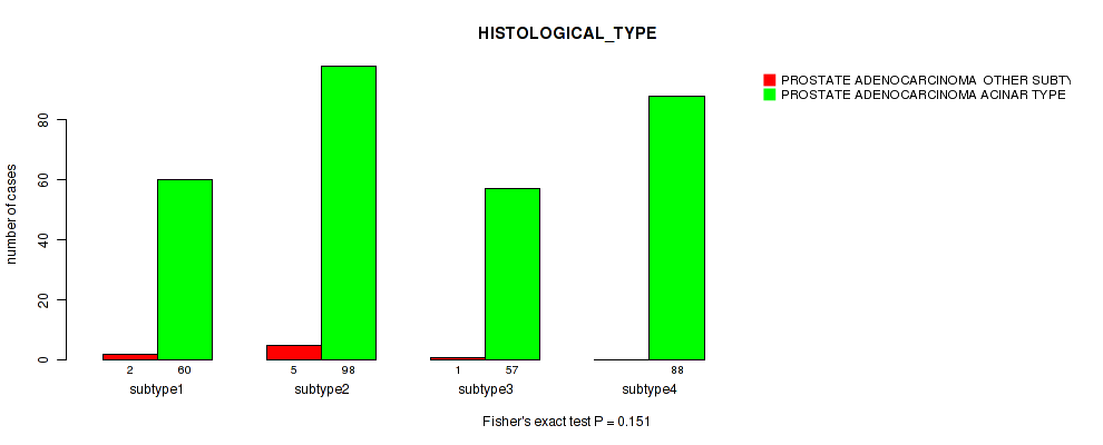
P value = 0.151 (Fisher's exact test), Q value = 0.22
Table S96. Clustering Approach #7: 'MIRseq Mature CNMF subtypes' versus Clinical Feature #5: 'HISTOLOGICAL_TYPE'
| nPatients | PROSTATE ADENOCARCINOMA OTHER SUBTYPE | PROSTATE ADENOCARCINOMA ACINAR TYPE |
|---|---|---|
| ALL | 8 | 303 |
| subtype1 | 2 | 60 |
| subtype2 | 5 | 98 |
| subtype3 | 1 | 57 |
| subtype4 | 0 | 88 |
Figure S89. Get High-res Image Clustering Approach #7: 'MIRseq Mature CNMF subtypes' versus Clinical Feature #5: 'HISTOLOGICAL_TYPE'
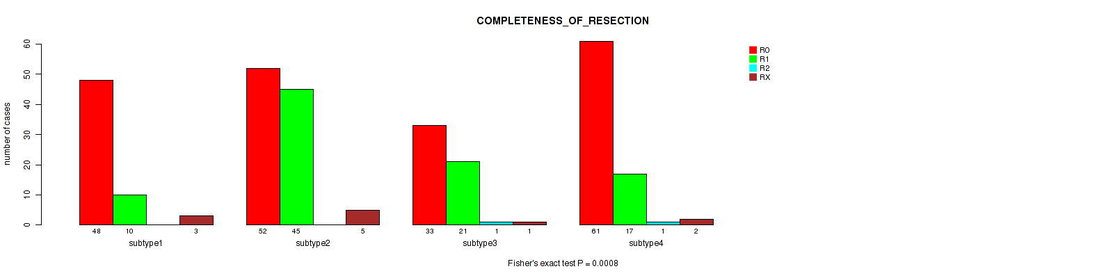
P value = 8e-04 (Fisher's exact test), Q value = 0.0022
Table S97. Clustering Approach #7: 'MIRseq Mature CNMF subtypes' versus Clinical Feature #6: 'COMPLETENESS_OF_RESECTION'
| nPatients | R0 | R1 | R2 | RX |
|---|---|---|---|---|
| ALL | 194 | 93 | 2 | 11 |
| subtype1 | 48 | 10 | 0 | 3 |
| subtype2 | 52 | 45 | 0 | 5 |
| subtype3 | 33 | 21 | 1 | 1 |
| subtype4 | 61 | 17 | 1 | 2 |
Figure S90. Get High-res Image Clustering Approach #7: 'MIRseq Mature CNMF subtypes' versus Clinical Feature #6: 'COMPLETENESS_OF_RESECTION'
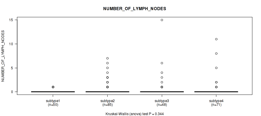
P value = 0.344 (Kruskal-Wallis (anova)), Q value = 0.43
Table S98. Clustering Approach #7: 'MIRseq Mature CNMF subtypes' versus Clinical Feature #7: 'NUMBER_OF_LYMPH_NODES'
| nPatients | Mean (Std.Dev) | |
|---|---|---|
| ALL | 254 | 0.5 (1.6) |
| subtype1 | 50 | 0.2 (0.4) |
| subtype2 | 85 | 0.5 (1.3) |
| subtype3 | 48 | 0.8 (2.4) |
| subtype4 | 71 | 0.4 (1.7) |
Figure S91. Get High-res Image Clustering Approach #7: 'MIRseq Mature CNMF subtypes' versus Clinical Feature #7: 'NUMBER_OF_LYMPH_NODES'
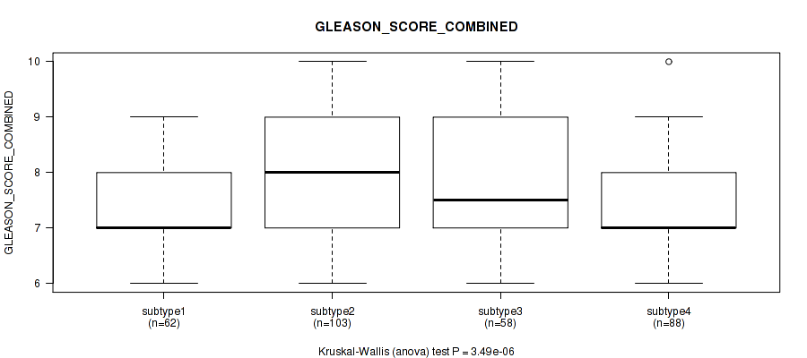
P value = 3.49e-06 (Kruskal-Wallis (anova)), Q value = 3e-05
Table S99. Clustering Approach #7: 'MIRseq Mature CNMF subtypes' versus Clinical Feature #8: 'GLEASON_SCORE_COMBINED'
| nPatients | Mean (Std.Dev) | |
|---|---|---|
| ALL | 311 | 7.6 (1.1) |
| subtype1 | 62 | 7.3 (0.9) |
| subtype2 | 103 | 8.0 (1.1) |
| subtype3 | 58 | 7.8 (1.3) |
| subtype4 | 88 | 7.3 (0.8) |
Figure S92. Get High-res Image Clustering Approach #7: 'MIRseq Mature CNMF subtypes' versus Clinical Feature #8: 'GLEASON_SCORE_COMBINED'
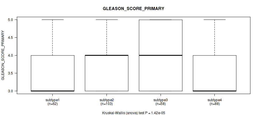
P value = 1.42e-05 (Kruskal-Wallis (anova)), Q value = 7.9e-05
Table S100. Clustering Approach #7: 'MIRseq Mature CNMF subtypes' versus Clinical Feature #9: 'GLEASON_SCORE_PRIMARY'
| nPatients | Mean (Std.Dev) | |
|---|---|---|
| ALL | 311 | 3.7 (0.7) |
| subtype1 | 62 | 3.5 (0.6) |
| subtype2 | 103 | 4.0 (0.7) |
| subtype3 | 58 | 3.9 (0.8) |
| subtype4 | 88 | 3.5 (0.6) |
Figure S93. Get High-res Image Clustering Approach #7: 'MIRseq Mature CNMF subtypes' versus Clinical Feature #9: 'GLEASON_SCORE_PRIMARY'
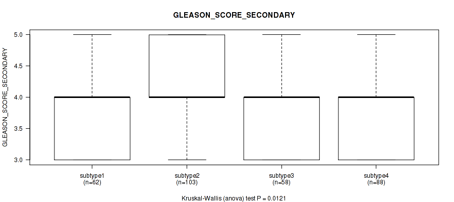
P value = 0.0121 (Kruskal-Wallis (anova)), Q value = 0.025
Table S101. Clustering Approach #7: 'MIRseq Mature CNMF subtypes' versus Clinical Feature #10: 'GLEASON_SCORE_SECONDARY'
| nPatients | Mean (Std.Dev) | |
|---|---|---|
| ALL | 311 | 3.9 (0.7) |
| subtype1 | 62 | 3.8 (0.7) |
| subtype2 | 103 | 4.1 (0.7) |
| subtype3 | 58 | 3.9 (0.7) |
| subtype4 | 88 | 3.8 (0.6) |
Figure S94. Get High-res Image Clustering Approach #7: 'MIRseq Mature CNMF subtypes' versus Clinical Feature #10: 'GLEASON_SCORE_SECONDARY'
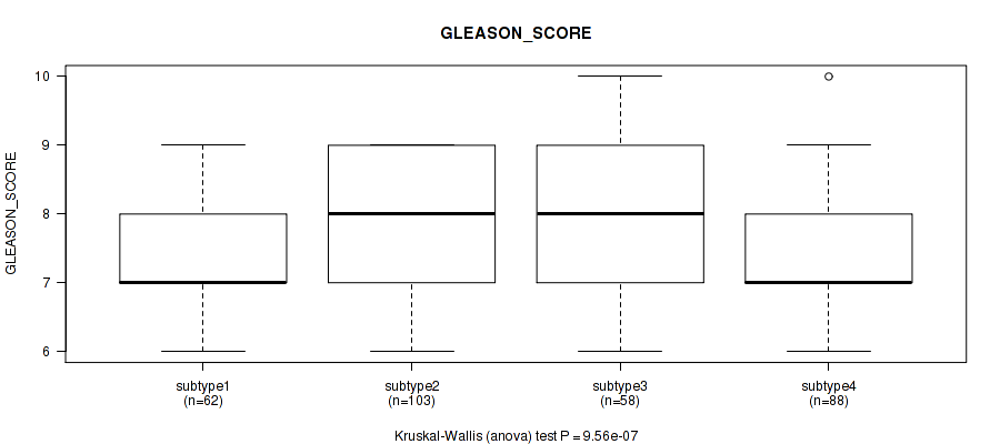
P value = 9.56e-07 (Kruskal-Wallis (anova)), Q value = 8.9e-06
Table S102. Clustering Approach #7: 'MIRseq Mature CNMF subtypes' versus Clinical Feature #11: 'GLEASON_SCORE'
| nPatients | Mean (Std.Dev) | |
|---|---|---|
| ALL | 311 | 7.6 (1.0) |
| subtype1 | 62 | 7.3 (1.0) |
| subtype2 | 103 | 8.0 (1.0) |
| subtype3 | 58 | 7.9 (1.2) |
| subtype4 | 88 | 7.3 (0.8) |
Figure S95. Get High-res Image Clustering Approach #7: 'MIRseq Mature CNMF subtypes' versus Clinical Feature #11: 'GLEASON_SCORE'
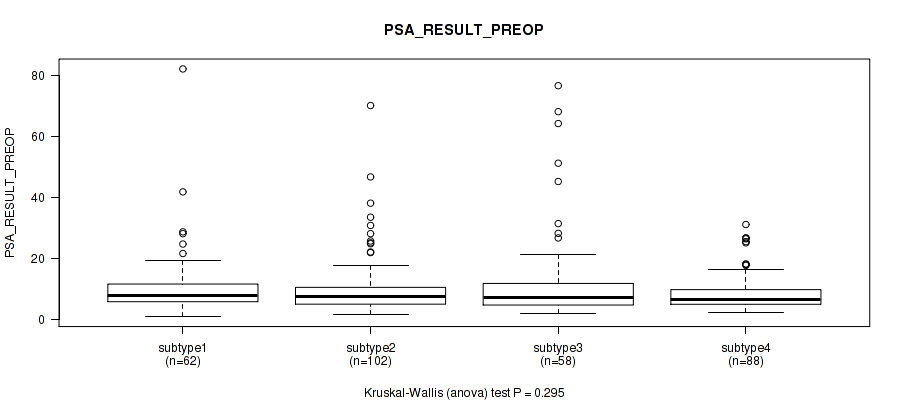
P value = 0.295 (Kruskal-Wallis (anova)), Q value = 0.38
Table S103. Clustering Approach #7: 'MIRseq Mature CNMF subtypes' versus Clinical Feature #12: 'PSA_RESULT_PREOP'
| nPatients | Mean (Std.Dev) | |
|---|---|---|
| ALL | 310 | 10.4 (11.0) |
| subtype1 | 62 | 11.0 (11.5) |
| subtype2 | 102 | 10.0 (9.8) |
| subtype3 | 58 | 13.3 (16.4) |
| subtype4 | 88 | 8.6 (6.2) |
Figure S96. Get High-res Image Clustering Approach #7: 'MIRseq Mature CNMF subtypes' versus Clinical Feature #12: 'PSA_RESULT_PREOP'
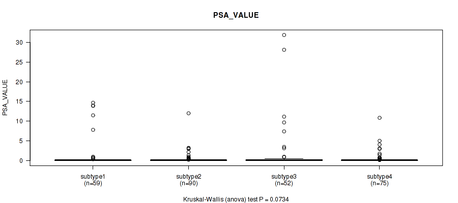
P value = 0.0734 (Kruskal-Wallis (anova)), Q value = 0.12
Table S104. Clustering Approach #7: 'MIRseq Mature CNMF subtypes' versus Clinical Feature #13: 'PSA_VALUE'
| nPatients | Mean (Std.Dev) | |
|---|---|---|
| ALL | 276 | 0.9 (3.3) |
| subtype1 | 59 | 1.2 (3.5) |
| subtype2 | 90 | 0.4 (1.4) |
| subtype3 | 52 | 1.9 (6.1) |
| subtype4 | 75 | 0.5 (1.5) |
Figure S97. Get High-res Image Clustering Approach #7: 'MIRseq Mature CNMF subtypes' versus Clinical Feature #13: 'PSA_VALUE'
P value = 0.805 (Fisher's exact test), Q value = 0.83
Table S105. Clustering Approach #7: 'MIRseq Mature CNMF subtypes' versus Clinical Feature #14: 'RACE'
| nPatients | ASIAN | BLACK OR AFRICAN AMERICAN | WHITE |
|---|---|---|---|
| ALL | 1 | 3 | 91 |
| subtype1 | 0 | 0 | 27 |
| subtype2 | 0 | 0 | 3 |
| subtype3 | 0 | 0 | 7 |
| subtype4 | 1 | 3 | 54 |
Figure S98. Get High-res Image Clustering Approach #7: 'MIRseq Mature CNMF subtypes' versus Clinical Feature #14: 'RACE'
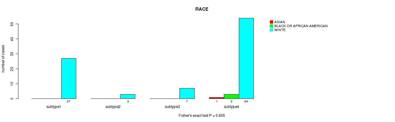
Table S106. Description of clustering approach #8: 'MIRseq Mature cHierClus subtypes'
| Cluster Labels | 1 | 2 | 3 | 4 | 5 | 6 |
|---|---|---|---|---|---|---|
| Number of samples | 68 | 40 | 35 | 83 | 25 | 60 |
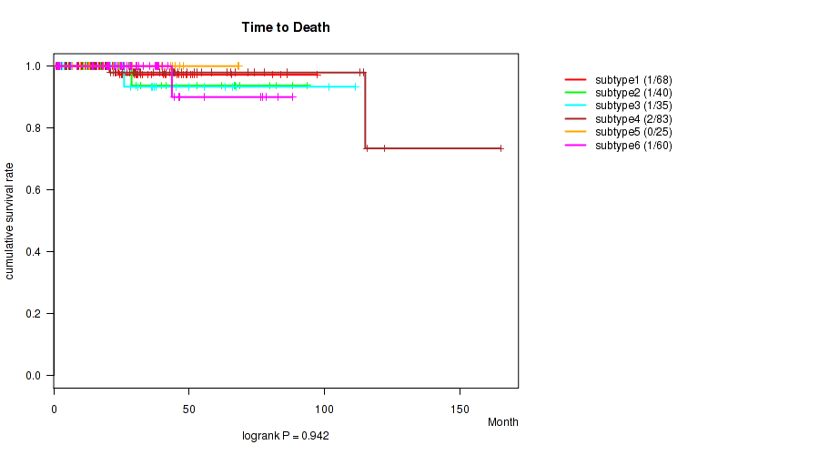
P value = 0.942 (logrank test), Q value = 0.95
Table S107. Clustering Approach #8: 'MIRseq Mature cHierClus subtypes' versus Clinical Feature #1: 'Time to Death'
| nPatients | nDeath | Duration Range (Median), Month | |
|---|---|---|---|
| ALL | 311 | 6 | 0.8 - 165.2 (25.4) |
| subtype1 | 68 | 1 | 1.2 - 97.4 (24.8) |
| subtype2 | 40 | 1 | 3.9 - 93.7 (26.2) |
| subtype3 | 35 | 1 | 2.0 - 111.4 (22.8) |
| subtype4 | 83 | 2 | 0.8 - 165.2 (27.2) |
| subtype5 | 25 | 0 | 1.0 - 68.3 (28.9) |
| subtype6 | 60 | 1 | 1.1 - 88.3 (26.0) |
Figure S99. Get High-res Image Clustering Approach #8: 'MIRseq Mature cHierClus subtypes' versus Clinical Feature #1: 'Time to Death'
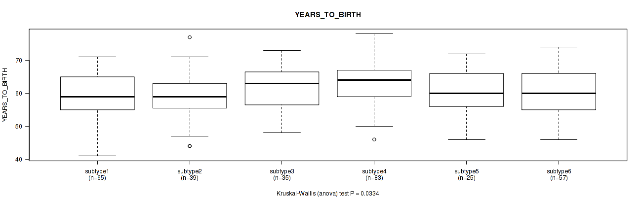
P value = 0.0334 (Kruskal-Wallis (anova)), Q value = 0.06
Table S108. Clustering Approach #8: 'MIRseq Mature cHierClus subtypes' versus Clinical Feature #2: 'YEARS_TO_BIRTH'
| nPatients | Mean (Std.Dev) | |
|---|---|---|
| ALL | 304 | 60.9 (7.0) |
| subtype1 | 65 | 59.7 (6.7) |
| subtype2 | 39 | 59.2 (7.0) |
| subtype3 | 35 | 61.7 (6.7) |
| subtype4 | 83 | 63.0 (6.6) |
| subtype5 | 25 | 60.3 (7.6) |
| subtype6 | 57 | 60.0 (7.2) |
Figure S100. Get High-res Image Clustering Approach #8: 'MIRseq Mature cHierClus subtypes' versus Clinical Feature #2: 'YEARS_TO_BIRTH'
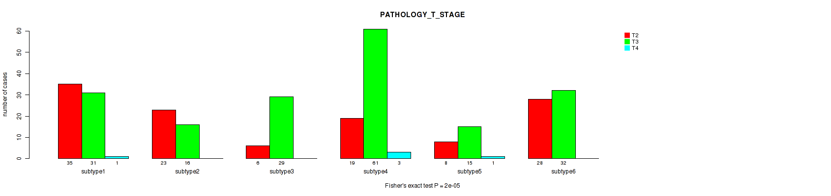
P value = 2e-05 (Fisher's exact test), Q value = 9.3e-05
Table S109. Clustering Approach #8: 'MIRseq Mature cHierClus subtypes' versus Clinical Feature #3: 'PATHOLOGY_T_STAGE'
| nPatients | T2 | T3 | T4 |
|---|---|---|---|
| ALL | 119 | 184 | 5 |
| subtype1 | 35 | 31 | 1 |
| subtype2 | 23 | 16 | 0 |
| subtype3 | 6 | 29 | 0 |
| subtype4 | 19 | 61 | 3 |
| subtype5 | 8 | 15 | 1 |
| subtype6 | 28 | 32 | 0 |
Figure S101. Get High-res Image Clustering Approach #8: 'MIRseq Mature cHierClus subtypes' versus Clinical Feature #3: 'PATHOLOGY_T_STAGE'
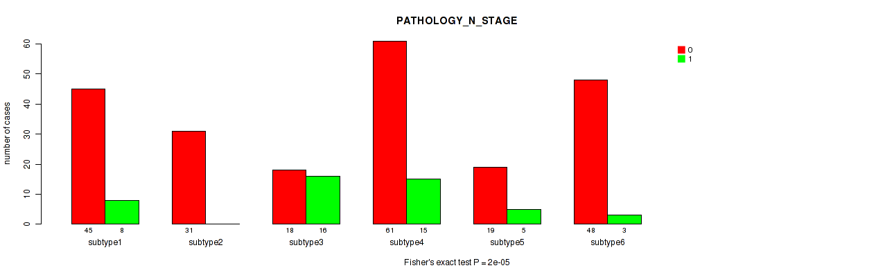
P value = 2e-05 (Fisher's exact test), Q value = 9.3e-05
Table S110. Clustering Approach #8: 'MIRseq Mature cHierClus subtypes' versus Clinical Feature #4: 'PATHOLOGY_N_STAGE'
| nPatients | 0 | 1 |
|---|---|---|
| ALL | 222 | 47 |
| subtype1 | 45 | 8 |
| subtype2 | 31 | 0 |
| subtype3 | 18 | 16 |
| subtype4 | 61 | 15 |
| subtype5 | 19 | 5 |
| subtype6 | 48 | 3 |
Figure S102. Get High-res Image Clustering Approach #8: 'MIRseq Mature cHierClus subtypes' versus Clinical Feature #4: 'PATHOLOGY_N_STAGE'
P value = 0.627 (Fisher's exact test), Q value = 0.71
Table S111. Clustering Approach #8: 'MIRseq Mature cHierClus subtypes' versus Clinical Feature #5: 'HISTOLOGICAL_TYPE'
| nPatients | PROSTATE ADENOCARCINOMA OTHER SUBTYPE | PROSTATE ADENOCARCINOMA ACINAR TYPE |
|---|---|---|
| ALL | 8 | 303 |
| subtype1 | 3 | 65 |
| subtype2 | 1 | 39 |
| subtype3 | 1 | 34 |
| subtype4 | 3 | 80 |
| subtype5 | 0 | 25 |
| subtype6 | 0 | 60 |
Figure S103. Get High-res Image Clustering Approach #8: 'MIRseq Mature cHierClus subtypes' versus Clinical Feature #5: 'HISTOLOGICAL_TYPE'
P value = 0.00043 (Fisher's exact test), Q value = 0.0013
Table S112. Clustering Approach #8: 'MIRseq Mature cHierClus subtypes' versus Clinical Feature #6: 'COMPLETENESS_OF_RESECTION'
| nPatients | R0 | R1 | R2 | RX |
|---|---|---|---|---|
| ALL | 194 | 93 | 2 | 11 |
| subtype1 | 52 | 10 | 0 | 4 |
| subtype2 | 27 | 11 | 1 | 0 |
| subtype3 | 16 | 17 | 0 | 2 |
| subtype4 | 42 | 38 | 0 | 2 |
| subtype5 | 17 | 7 | 0 | 1 |
| subtype6 | 40 | 10 | 1 | 2 |
Figure S104. Get High-res Image Clustering Approach #8: 'MIRseq Mature cHierClus subtypes' versus Clinical Feature #6: 'COMPLETENESS_OF_RESECTION'
P value = 4.35e-07 (Kruskal-Wallis (anova)), Q value = 4.4e-06
Table S113. Clustering Approach #8: 'MIRseq Mature cHierClus subtypes' versus Clinical Feature #7: 'NUMBER_OF_LYMPH_NODES'
| nPatients | Mean (Std.Dev) | |
|---|---|---|
| ALL | 254 | 0.5 (1.6) |
| subtype1 | 45 | 0.2 (0.7) |
| subtype2 | 30 | 0.0 (0.0) |
| subtype3 | 31 | 2.0 (3.6) |
| subtype4 | 73 | 0.5 (1.4) |
| subtype5 | 24 | 0.2 (0.4) |
| subtype6 | 51 | 0.1 (0.3) |
Figure S105. Get High-res Image Clustering Approach #8: 'MIRseq Mature cHierClus subtypes' versus Clinical Feature #7: 'NUMBER_OF_LYMPH_NODES'
P value = 1.43e-10 (Kruskal-Wallis (anova)), Q value = 2.3e-09
Table S114. Clustering Approach #8: 'MIRseq Mature cHierClus subtypes' versus Clinical Feature #8: 'GLEASON_SCORE_COMBINED'
| nPatients | Mean (Std.Dev) | |
|---|---|---|
| ALL | 311 | 7.6 (1.1) |
| subtype1 | 68 | 7.5 (1.0) |
| subtype2 | 40 | 7.0 (1.2) |
| subtype3 | 35 | 8.3 (1.0) |
| subtype4 | 83 | 8.1 (1.1) |
| subtype5 | 25 | 7.3 (0.8) |
| subtype6 | 60 | 7.3 (0.8) |
Figure S106. Get High-res Image Clustering Approach #8: 'MIRseq Mature cHierClus subtypes' versus Clinical Feature #8: 'GLEASON_SCORE_COMBINED'
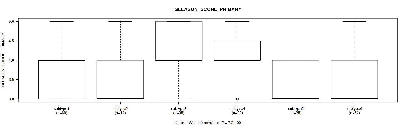
P value = 7.2e-09 (Kruskal-Wallis (anova)), Q value = 1e-07
Table S115. Clustering Approach #8: 'MIRseq Mature cHierClus subtypes' versus Clinical Feature #9: 'GLEASON_SCORE_PRIMARY'
| nPatients | Mean (Std.Dev) | |
|---|---|---|
| ALL | 311 | 3.7 (0.7) |
| subtype1 | 68 | 3.7 (0.6) |
| subtype2 | 40 | 3.4 (0.7) |
| subtype3 | 35 | 4.1 (0.8) |
| subtype4 | 83 | 4.0 (0.7) |
| subtype5 | 25 | 3.4 (0.5) |
| subtype6 | 60 | 3.5 (0.5) |
Figure S107. Get High-res Image Clustering Approach #8: 'MIRseq Mature cHierClus subtypes' versus Clinical Feature #9: 'GLEASON_SCORE_PRIMARY'
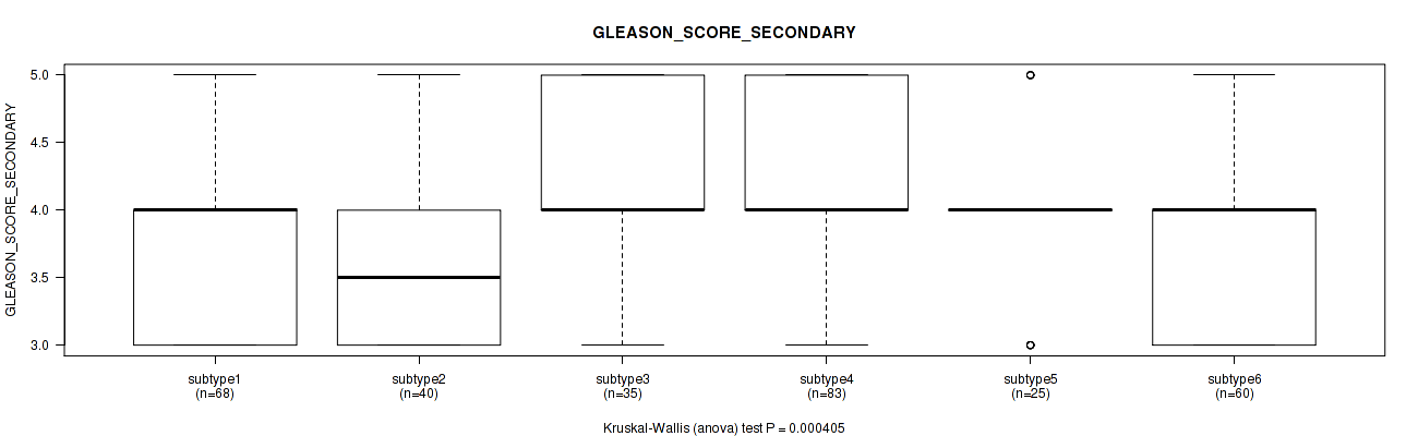
P value = 0.000405 (Kruskal-Wallis (anova)), Q value = 0.0013
Table S116. Clustering Approach #8: 'MIRseq Mature cHierClus subtypes' versus Clinical Feature #10: 'GLEASON_SCORE_SECONDARY'
| nPatients | Mean (Std.Dev) | |
|---|---|---|
| ALL | 311 | 3.9 (0.7) |
| subtype1 | 68 | 3.8 (0.7) |
| subtype2 | 40 | 3.6 (0.7) |
| subtype3 | 35 | 4.1 (0.7) |
| subtype4 | 83 | 4.1 (0.7) |
| subtype5 | 25 | 3.9 (0.6) |
| subtype6 | 60 | 3.8 (0.6) |
Figure S108. Get High-res Image Clustering Approach #8: 'MIRseq Mature cHierClus subtypes' versus Clinical Feature #10: 'GLEASON_SCORE_SECONDARY'
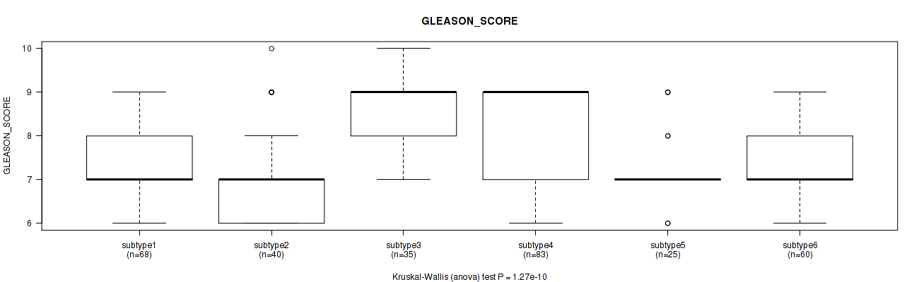
P value = 1.27e-10 (Kruskal-Wallis (anova)), Q value = 2.3e-09
Table S117. Clustering Approach #8: 'MIRseq Mature cHierClus subtypes' versus Clinical Feature #11: 'GLEASON_SCORE'
| nPatients | Mean (Std.Dev) | |
|---|---|---|
| ALL | 311 | 7.6 (1.0) |
| subtype1 | 68 | 7.5 (1.0) |
| subtype2 | 40 | 7.1 (1.1) |
| subtype3 | 35 | 8.4 (0.8) |
| subtype4 | 83 | 8.1 (1.0) |
| subtype5 | 25 | 7.2 (0.8) |
| subtype6 | 60 | 7.3 (0.8) |
Figure S109. Get High-res Image Clustering Approach #8: 'MIRseq Mature cHierClus subtypes' versus Clinical Feature #11: 'GLEASON_SCORE'
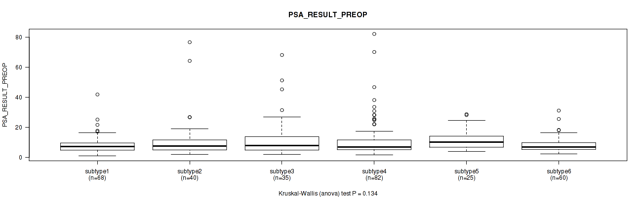
P value = 0.134 (Kruskal-Wallis (anova)), Q value = 0.2
Table S118. Clustering Approach #8: 'MIRseq Mature cHierClus subtypes' versus Clinical Feature #12: 'PSA_RESULT_PREOP'
| nPatients | Mean (Std.Dev) | |
|---|---|---|
| ALL | 310 | 10.4 (11.0) |
| subtype1 | 68 | 8.1 (6.0) |
| subtype2 | 40 | 11.7 (14.8) |
| subtype3 | 35 | 13.4 (15.0) |
| subtype4 | 82 | 11.6 (13.5) |
| subtype5 | 25 | 11.8 (7.0) |
| subtype6 | 60 | 8.2 (5.3) |
Figure S110. Get High-res Image Clustering Approach #8: 'MIRseq Mature cHierClus subtypes' versus Clinical Feature #12: 'PSA_RESULT_PREOP'
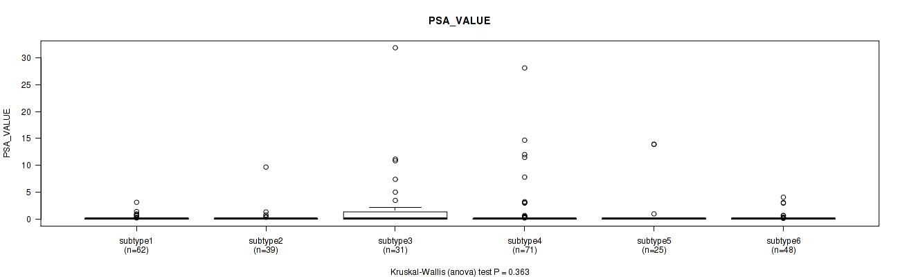
P value = 0.363 (Kruskal-Wallis (anova)), Q value = 0.44
Table S119. Clustering Approach #8: 'MIRseq Mature cHierClus subtypes' versus Clinical Feature #13: 'PSA_VALUE'
| nPatients | Mean (Std.Dev) | |
|---|---|---|
| ALL | 276 | 0.9 (3.3) |
| subtype1 | 62 | 0.2 (0.5) |
| subtype2 | 39 | 0.4 (1.5) |
| subtype3 | 31 | 2.5 (6.2) |
| subtype4 | 71 | 1.3 (4.2) |
| subtype5 | 25 | 1.2 (3.8) |
| subtype6 | 48 | 0.3 (0.8) |
Figure S111. Get High-res Image Clustering Approach #8: 'MIRseq Mature cHierClus subtypes' versus Clinical Feature #13: 'PSA_VALUE'
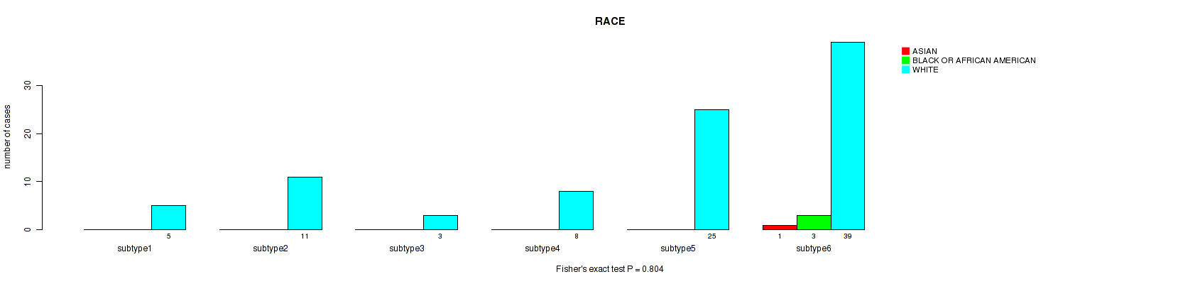
P value = 0.804 (Fisher's exact test), Q value = 0.83
Table S120. Clustering Approach #8: 'MIRseq Mature cHierClus subtypes' versus Clinical Feature #14: 'RACE'
| nPatients | ASIAN | BLACK OR AFRICAN AMERICAN | WHITE |
|---|---|---|---|
| ALL | 1 | 3 | 91 |
| subtype1 | 0 | 0 | 5 |
| subtype2 | 0 | 0 | 11 |
| subtype3 | 0 | 0 | 3 |
| subtype4 | 0 | 0 | 8 |
| subtype5 | 0 | 0 | 25 |
| subtype6 | 1 | 3 | 39 |
Figure S112. Get High-res Image Clustering Approach #8: 'MIRseq Mature cHierClus subtypes' versus Clinical Feature #14: 'RACE'
-
Cluster data file = /xchip/cga/gdac-prod/tcga-gdac/jobResults/GDAC_mergedClustering/PRAD-TP/15115159/PRAD-TP.mergedcluster.txt
-
Clinical data file = /xchip/cga/gdac-prod/tcga-gdac/jobResults/Append_Data/PRAD-TP/15087329/PRAD-TP.merged_data.txt
-
Number of patients = 488
-
Number of clustering approaches = 8
-
Number of selected clinical features = 14
-
Exclude small clusters that include fewer than K patients, K = 3
consensus non-negative matrix factorization clustering approach (Brunet et al. 2004)
Resampling-based clustering method (Monti et al. 2003)
For survival clinical features, the Kaplan-Meier survival curves of tumors with and without gene mutations were plotted and the statistical significance P values were estimated by logrank test (Bland and Altman 2004) using the 'survdiff' function in R
For binary clinical features, two-tailed Fisher's exact tests (Fisher 1922) were used to estimate the P values using the 'fisher.test' function in R
For multiple hypothesis correction, Q value is the False Discovery Rate (FDR) analogue of the P value (Benjamini and Hochberg 1995), defined as the minimum FDR at which the test may be called significant. We used the 'Benjamini and Hochberg' method of 'p.adjust' function in R to convert P values into Q values.
In addition to the links below, the full results of the analysis summarized in this report can also be downloaded programmatically using firehose_get, or interactively from either the Broad GDAC website or TCGA Data Coordination Center Portal.