This report serves to describe the mutational landscape and properties of a given individual set, as well as rank genes and genesets according to mutational significance. MutSig 2CV v3.1 was used to generate the results found in this report.
-
Working with individual set: KIRP-TP
-
Number of patients in set: 161
The input for this pipeline is a set of individuals with the following files associated for each:
-
An annotated .maf file describing the mutations called for the respective individual, and their properties.
-
A .wig file that contains information about the coverage of the sample.
-
MAF used for this analysis:KIRP-TP.final_analysis_set.maf
-
Blacklist used for this analysis: pancan_mutation_blacklist.v14.hg19.txt
-
Significantly mutated genes (q ≤ 0.1): 14
The mutation spectrum is depicted in the lego plots below in which the 96 possible mutation types are subdivided into six large blocks, color-coded to reflect the base substitution type. Each large block is further subdivided into the 16 possible pairs of 5' and 3' neighbors, as listed in the 4x4 trinucleotide context legend. The height of each block corresponds to the mutation frequency for that kind of mutation (counts of mutations normalized by the base coverage in a given bin). The shape of the spectrum is a signature for dominant mutational mechanisms in different tumor types.
Figure 1. Get High-res Image SNV Mutation rate lego plot for entire set. Each bin is normalized by base coverage for that bin. Colors represent the six SNV types on the upper right. The three-base context for each mutation is labeled in the 4x4 legend on the lower right. The fractional breakdown of SNV counts is shown in the pie chart on the upper left. If this figure is blank, not enough information was provided in the MAF to generate it.
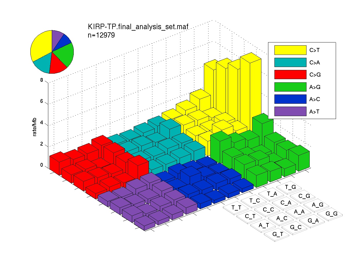
Figure 2. Get High-res Image SNV Mutation rate lego plots for 4 slices of mutation allele fraction (0<=AF<0.1, 0.1<=AF<0.25, 0.25<=AF<0.5, & 0.5<=AF) . The color code and three-base context legends are the same as the previous figure. If this figure is blank, not enough information was provided in the MAF to generate it.

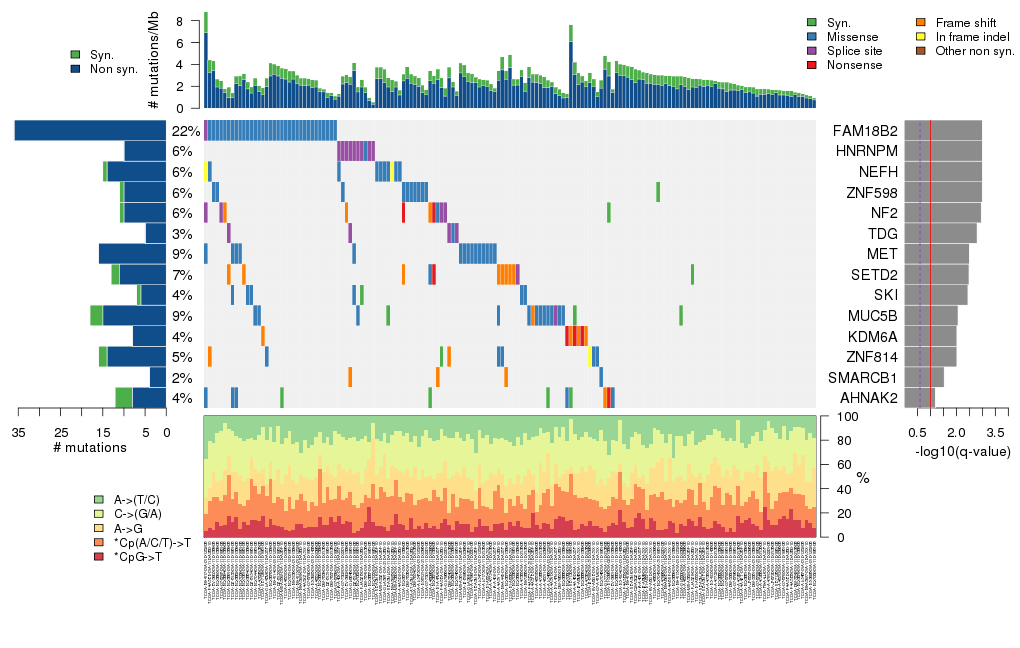
Figure 3. Get High-res Image The matrix in the center of the figure represents individual mutations in patient samples, color-coded by type of mutation, for the significantly mutated genes. The rate of synonymous and non-synonymous mutations is displayed at the top of the matrix. The barplot on the left of the matrix shows the number of mutations in each gene. The percentages represent the fraction of tumors with at least one mutation in the specified gene. The barplot to the right of the matrix displays the q-values for the most significantly mutated genes. The purple boxplots below the matrix (only displayed if required columns are present in the provided MAF) represent the distributions of allelic fractions observed in each sample. The plot at the bottom represents the base substitution distribution of individual samples, using the same categories that were used to calculate significance.
Column Descriptions:
-
nnon = number of (nonsilent) mutations in this gene across the individual set
-
npat = number of patients (individuals) with at least one nonsilent mutation
-
nsite = number of unique sites having a non-silent mutation
-
nsil = number of silent mutations in this gene across the individual set
-
p = p-value (overall)
-
q = q-value, False Discovery Rate (Benjamini-Hochberg procedure)
Table 1. Get Full Table A Ranked List of Significantly Mutated Genes. Number of significant genes found: 14. Number of genes displayed: 35. Click on a gene name to display its stick figure depicting the distribution of mutations and mutation types across the chosen gene (this feature may not be available for all significant genes).
| rank | gene | longname | codelen | nnei | nncd | nsil | nmis | nstp | nspl | nind | nnon | npat | nsite | pCV | pCL | pFN | p | q |
|---|---|---|---|---|---|---|---|---|---|---|---|---|---|---|---|---|---|---|
| 1 | FAM18B2 | family with sequence similarity 18, member B2 | 1003 | 101 | 0 | 0 | 35 | 0 | 1 | 0 | 36 | 35 | 2 | 1e-16 | 1e-05 | 0.83 | 1e-16 | 1.8e-12 |
| 2 | HNRNPM | heterogeneous nuclear ribonucleoprotein M | 2255 | 94 | 0 | 0 | 1 | 0 | 9 | 0 | 10 | 10 | 2 | 2.4e-10 | 1e-05 | 0.039 | 8.5e-14 | 7.7e-10 |
| 3 | NEFH | neurofilament, heavy polypeptide 200kDa | 3077 | 3 | 0 | 1 | 9 | 0 | 0 | 5 | 14 | 10 | 6 | 3.7e-07 | 1e-05 | 0.98 | 1e-10 | 6.2e-07 |
| 4 | ZNF598 | zinc finger protein 598 | 2763 | 36 | 0 | 1 | 10 | 0 | 0 | 0 | 10 | 10 | 1 | 7e-06 | 1e-05 | 1 | 1.7e-09 | 7.8e-06 |
| 5 | NF2 | neurofibromin 2 (merlin) | 1894 | 12 | 0 | 1 | 1 | 2 | 3 | 4 | 10 | 10 | 10 | 1.3e-09 | 1 | 0.89 | 2.8e-08 | 0.0001 |
| 6 | TDG | thymine-DNA glycosylase | 1269 | 128 | 0 | 0 | 1 | 0 | 4 | 0 | 5 | 5 | 3 | 2.8e-06 | 0.0036 | 0.24 | 2e-07 | 0.0006 |
| 7 | MET | met proto-oncogene (hepatocyte growth factor receptor) | 4307 | 15 | 0 | 0 | 15 | 0 | 0 | 1 | 16 | 15 | 14 | 0.00065 | 0.0031 | 0.0038 | 8.1e-07 | 0.0021 |
| 8 | SETD2 | SET domain containing 2 | 7777 | 25 | 0 | 2 | 1 | 1 | 1 | 8 | 11 | 11 | 11 | 5.6e-08 | 1 | 0.56 | 1e-06 | 0.0023 |
| 9 | SKI | v-ski sarcoma viral oncogene homolog (avian) | 2213 | 32 | 0 | 1 | 6 | 0 | 0 | 0 | 6 | 6 | 1 | 0.00053 | 2e-05 | 0.97 | 1.3e-06 | 0.0026 |
| 10 | MUC5B | mucin 5B, oligomeric mucus/gel-forming | 17492 | 26 | 0 | 3 | 13 | 0 | 1 | 1 | 15 | 14 | 11 | 0.026 | 1e-05 | 0.68 | 4.2e-06 | 0.0076 |
| 11 | KDM6A | lysine (K)-specific demethylase 6A | 4318 | 37 | 0 | 0 | 0 | 3 | 1 | 4 | 8 | 7 | 8 | 3.5e-07 | 1 | 0.74 | 5.5e-06 | 0.0087 |
| 12 | ZNF814 | zinc finger protein 814 | 2576 | 5 | 0 | 2 | 11 | 0 | 0 | 3 | 14 | 8 | 8 | 0.036 | 1e-05 | 0.91 | 5.7e-06 | 0.0087 |
| 13 | SMARCB1 | SWI/SNF related, matrix associated, actin dependent regulator of chromatin, subfamily b, member 1 | 1190 | 0 | 0 | 0 | 1 | 0 | 0 | 3 | 4 | 4 | 3 | 0.000063 | 0.019 | 0.77 | 2e-05 | 0.028 |
| 14 | AHNAK2 | AHNAK nucleoprotein 2 | 17412 | 22 | 0 | 4 | 6 | 1 | 0 | 1 | 8 | 7 | 6 | 0.36 | 1e-05 | 0.18 | 0.000048 | 0.063 |
| 15 | OR2L8 | olfactory receptor, family 2, subfamily L, member 8 | 939 | 76 | 0 | 1 | 1 | 0 | 0 | 3 | 4 | 4 | 2 | 0.065 | 0.0001 | 0.95 | 0.000084 | 0.1 |
| 16 | PAM | peptidylglycine alpha-amidating monooxygenase | 3021 | 7 | 0 | 0 | 3 | 0 | 0 | 2 | 5 | 3 | 5 | 0.15 | 4e-05 | 0.48 | 0.00012 | 0.13 |
| 17 | IDUA | iduronidase, alpha-L- | 2074 | 138 | 0 | 0 | 5 | 0 | 0 | 0 | 5 | 5 | 2 | 0.0032 | 0.0015 | 0.99 | 0.00012 | 0.13 |
| 18 | CSGALNACT2 | chondroitin sulfate N-acetylgalactosaminyltransferase 2 | 1653 | 26 | 0 | 1 | 5 | 0 | 0 | 0 | 5 | 5 | 2 | 0.036 | 0.00017 | 0.82 | 0.00014 | 0.14 |
| 19 | RPL7A | ribosomal protein L7a | 995 | 12 | 0 | 0 | 1 | 0 | 2 | 0 | 3 | 3 | 2 | 0.0014 | 0.031 | 0.077 | 0.00027 | 0.26 |
| 20 | HOXD8 | homeobox D8 | 877 | 33 | 0 | 0 | 2 | 0 | 0 | 2 | 4 | 4 | 3 | 0.00066 | 0.033 | 0.97 | 0.00029 | 0.27 |
| 21 | BMS1 | BMS1 homolog, ribosome assembly protein (yeast) | 3937 | 66 | 0 | 1 | 4 | 0 | 0 | 0 | 4 | 4 | 2 | 0.28 | 0.0001 | 0.94 | 0.00032 | 0.28 |
| 22 | C14orf126 | chromosome 14 open reading frame 126 | 517 | 263 | 0 | 0 | 5 | 0 | 0 | 0 | 5 | 5 | 1 | 0.000085 | 0.29 | 1 | 0.00038 | 0.31 |
| 23 | SLC6A13 | solute carrier family 6 (neurotransmitter transporter, GABA), member 13 | 1865 | 57 | 0 | 0 | 4 | 0 | 0 | 0 | 4 | 4 | 4 | 0.00036 | 1 | 0.078 | 0.0004 | 0.31 |
| 24 | CUL3 | cullin 3 | 2367 | 3 | 0 | 0 | 4 | 2 | 0 | 1 | 7 | 5 | 7 | 0.0011 | 0.03 | 1 | 0.00045 | 0.32 |
| 25 | BHMT | betaine-homocysteine methyltransferase | 1249 | 285 | 0 | 0 | 3 | 0 | 1 | 1 | 5 | 5 | 5 | 0.00053 | 1 | 0.053 | 0.00045 | 0.32 |
| 26 | KCNK5 | potassium channel, subfamily K, member 5 | 1516 | 69 | 0 | 0 | 0 | 1 | 1 | 1 | 3 | 3 | 3 | 0.00041 | 1 | 0.081 | 0.00046 | 0.32 |
| 27 | LGI4 | leucine-rich repeat LGI family, member 4 | 1646 | 220 | 0 | 0 | 4 | 0 | 0 | 0 | 4 | 4 | 4 | 0.0012 | 1 | 0.011 | 0.00054 | 0.36 |
| 28 | GAGE2A | G antigen 2A | 1486 | 55 | 0 | 0 | 0 | 0 | 0 | 2 | 2 | 2 | 1 | 0.0051 | 0.01 | 0.7 | 0.00056 | 0.36 |
| 29 | LOC441294 | 2335 | 121 | 0 | 0 | 2 | 0 | 0 | 0 | 2 | 2 | 1 | 0.0054 | 0.017 | 0.01 | 0.00059 | 0.37 | |
| 30 | ACADL | acyl-Coenzyme A dehydrogenase, long chain | 1333 | 183 | 0 | 0 | 2 | 0 | 1 | 1 | 4 | 3 | 4 | 0.0089 | 0.013 | 0.25 | 0.0007 | 0.42 |
| 31 | HLA-B | major histocompatibility complex, class I, B | 1119 | 9 | 0 | 1 | 0 | 0 | 1 | 1 | 2 | 2 | 2 | 0.0049 | 1 | 0.01 | 0.0009 | 0.53 |
| 32 | TMCO3 | transmembrane and coiled-coil domains 3 | 2082 | 3 | 0 | 0 | 0 | 0 | 0 | 2 | 2 | 2 | 1 | 0.0092 | 0.01 | 0.28 | 0.00095 | 0.54 |
| 33 | SAV1 | salvador homolog 1 (Drosophila) | 1168 | 236 | 0 | 0 | 2 | 0 | 0 | 3 | 5 | 5 | 5 | 0.00011 | 1 | 1 | 0.0011 | 0.62 |
| 34 | ORC2L | origin recognition complex, subunit 2-like (yeast) | 1798 | 14 | 0 | 0 | 2 | 1 | 0 | 1 | 4 | 4 | 4 | 0.0019 | 1 | 0.058 | 0.0012 | 0.63 |
| 35 | AHCY | S-adenosylhomocysteine hydrolase | 1335 | 22 | 0 | 1 | 2 | 0 | 1 | 1 | 4 | 4 | 4 | 0.00012 | 1 | 0.76 | 0.0012 | 0.63 |
Figure S1. This figure depicts the distribution of mutations and mutation types across the HNRNPM significant gene.
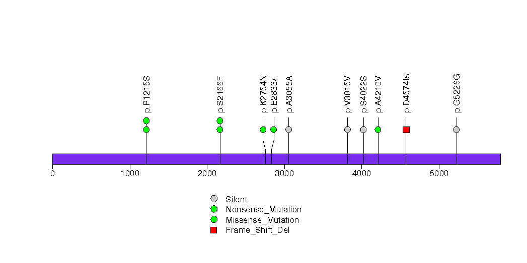
Figure S2. This figure depicts the distribution of mutations and mutation types across the NEFH significant gene.
Figure S3. This figure depicts the distribution of mutations and mutation types across the ZNF598 significant gene.
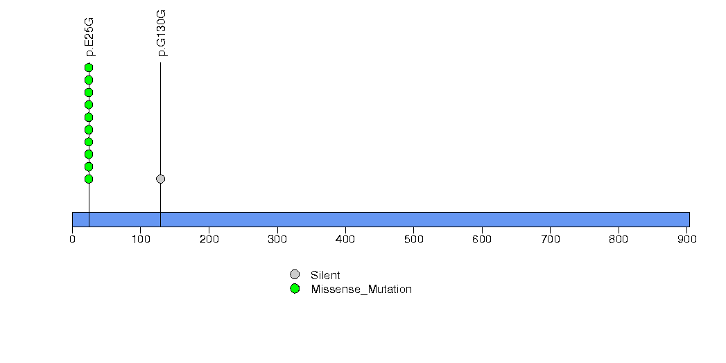
Figure S4. This figure depicts the distribution of mutations and mutation types across the NF2 significant gene.
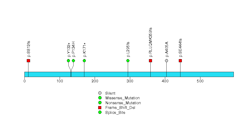
Figure S5. This figure depicts the distribution of mutations and mutation types across the TDG significant gene.
Figure S6. This figure depicts the distribution of mutations and mutation types across the MET significant gene.
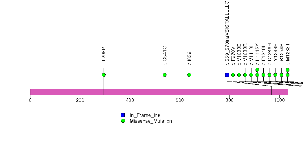
Figure S7. This figure depicts the distribution of mutations and mutation types across the SETD2 significant gene.
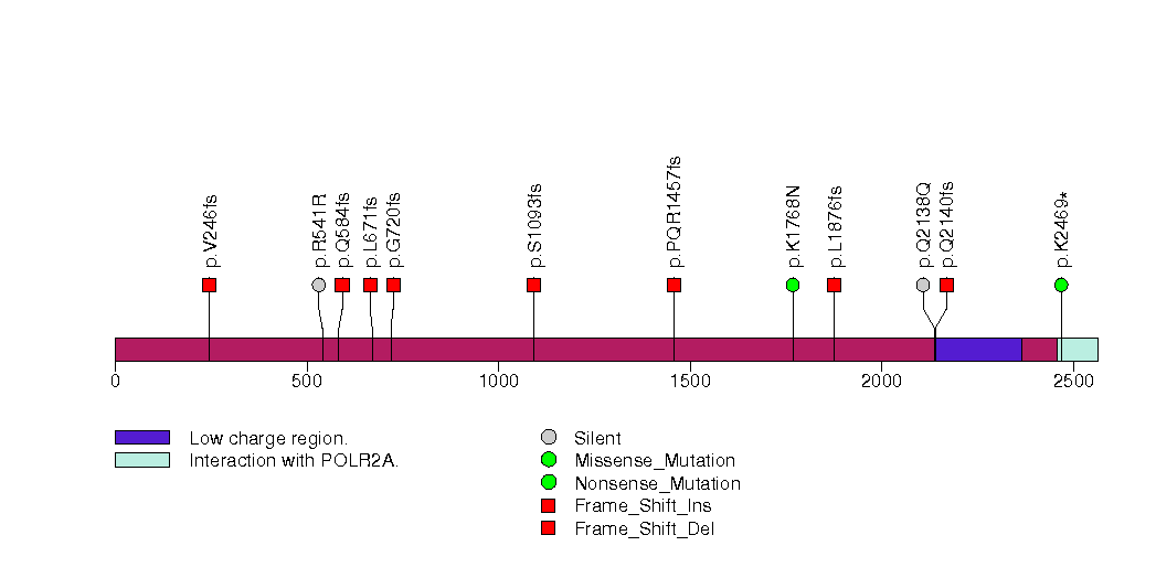
Figure S8. This figure depicts the distribution of mutations and mutation types across the SKI significant gene.
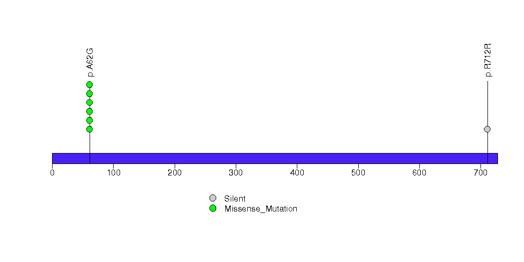
Figure S9. This figure depicts the distribution of mutations and mutation types across the MUC5B significant gene.
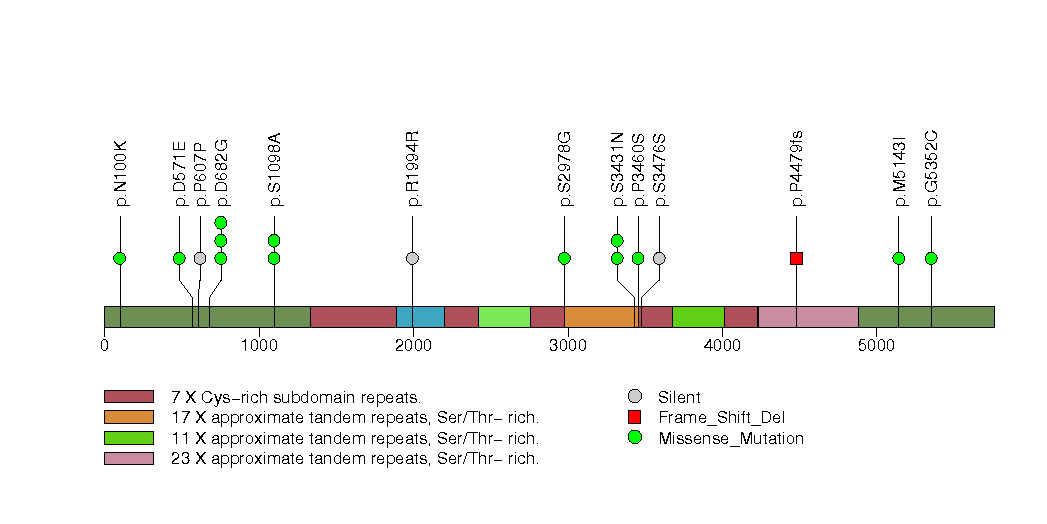
Figure S10. This figure depicts the distribution of mutations and mutation types across the KDM6A significant gene.
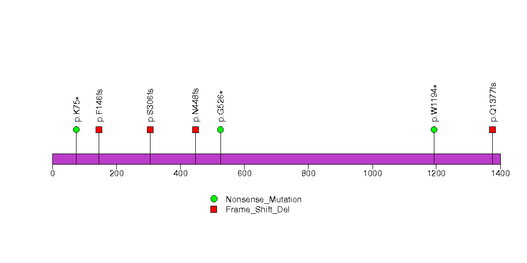
Figure S11. This figure depicts the distribution of mutations and mutation types across the ZNF814 significant gene.
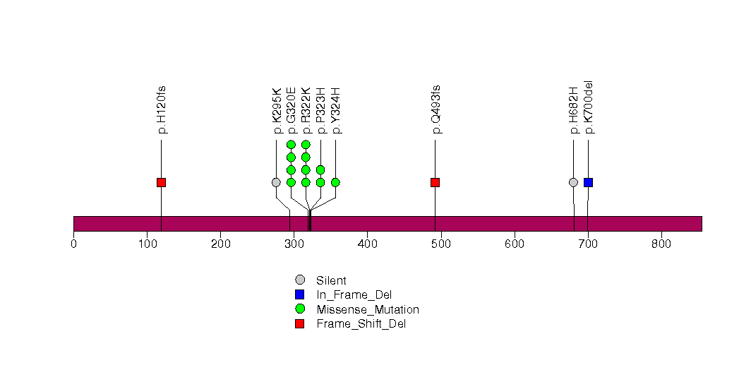
Figure S12. This figure depicts the distribution of mutations and mutation types across the SMARCB1 significant gene.
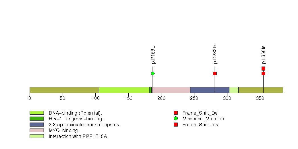
Figure S13. This figure depicts the distribution of mutations and mutation types across the AHNAK2 significant gene.
In brief, we tabulate the number of mutations and the number of covered bases for each gene. The counts are broken down by mutation context category: four context categories that are discovered by MutSig, and one for indel and 'null' mutations, which include indels, nonsense mutations, splice-site mutations, and non-stop (read-through) mutations. For each gene, we calculate the probability of seeing the observed constellation of mutations, i.e. the product P1 x P2 x ... x Pm, or a more extreme one, given the background mutation rates calculated across the dataset. [1]
In addition to the links below, the full results of the analysis summarized in this report can also be downloaded programmatically using firehose_get, or interactively from either the Broad GDAC website or TCGA Data Coordination Center Portal.