This report serves to describe the mutational landscape and properties of a given individual set, as well as rank genes and genesets according to mutational significance. MutSig 2CV v3.1 was used to generate the results found in this report.
-
Working with individual set: THYM-TP
-
Number of patients in set: 120
The input for this pipeline is a set of individuals with the following files associated for each:
-
An annotated .maf file describing the mutations called for the respective individual, and their properties.
-
A .wig file that contains information about the coverage of the sample.
-
MAF used for this analysis:THYM-TP.final_analysis_set.maf
-
Blacklist used for this analysis: pancan_mutation_blacklist.v14.hg19.txt
-
Significantly mutated genes (q ≤ 0.1): 8
The mutation spectrum is depicted in the lego plots below in which the 96 possible mutation types are subdivided into six large blocks, color-coded to reflect the base substitution type. Each large block is further subdivided into the 16 possible pairs of 5' and 3' neighbors, as listed in the 4x4 trinucleotide context legend. The height of each block corresponds to the mutation frequency for that kind of mutation (counts of mutations normalized by the base coverage in a given bin). The shape of the spectrum is a signature for dominant mutational mechanisms in different tumor types.
Figure 1. Get High-res Image SNV Mutation rate lego plot for entire set. Each bin is normalized by base coverage for that bin. Colors represent the six SNV types on the upper right. The three-base context for each mutation is labeled in the 4x4 legend on the lower right. The fractional breakdown of SNV counts is shown in the pie chart on the upper left. If this figure is blank, not enough information was provided in the MAF to generate it.
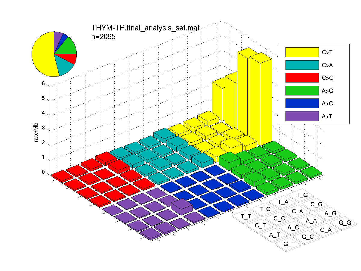
Figure 2. Get High-res Image SNV Mutation rate lego plots for 4 slices of mutation allele fraction (0<=AF<0.1, 0.1<=AF<0.25, 0.25<=AF<0.5, & 0.5<=AF) . The color code and three-base context legends are the same as the previous figure. If this figure is blank, not enough information was provided in the MAF to generate it.

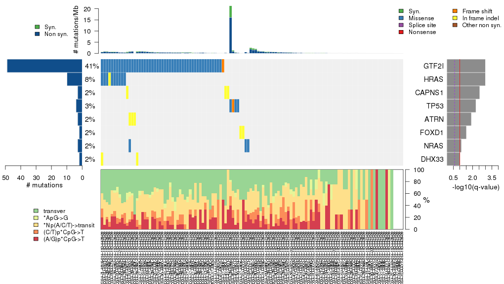
Figure 3. Get High-res Image The matrix in the center of the figure represents individual mutations in patient samples, color-coded by type of mutation, for the significantly mutated genes. The rate of synonymous and non-synonymous mutations is displayed at the top of the matrix. The barplot on the left of the matrix shows the number of mutations in each gene. The percentages represent the fraction of tumors with at least one mutation in the specified gene. The barplot to the right of the matrix displays the q-values for the most significantly mutated genes. The purple boxplots below the matrix (only displayed if required columns are present in the provided MAF) represent the distributions of allelic fractions observed in each sample. The plot at the bottom represents the base substitution distribution of individual samples, using the same categories that were used to calculate significance.
Column Descriptions:
-
nnon = number of (nonsilent) mutations in this gene across the individual set
-
npat = number of patients (individuals) with at least one nonsilent mutation
-
nsite = number of unique sites having a non-silent mutation
-
nsil = number of silent mutations in this gene across the individual set
-
p = p-value (overall)
-
q = q-value, False Discovery Rate (Benjamini-Hochberg procedure)
Table 1. Get Full Table A Ranked List of Significantly Mutated Genes. Number of significant genes found: 8. Number of genes displayed: 35. Click on a gene name to display its stick figure depicting the distribution of mutations and mutation types across the chosen gene (this feature may not be available for all significant genes).
| rank | gene | longname | codelen | nnei | nncd | nsil | nmis | nstp | nspl | nind | nnon | npat | nsite | pCV | pCL | pFN | p | q |
|---|---|---|---|---|---|---|---|---|---|---|---|---|---|---|---|---|---|---|
| 1 | GTF2I | general transcription factor II, i | 3133 | 813 | 0 | 0 | 48 | 0 | 0 | 1 | 49 | 49 | 2 | 2.3e-15 | 1e-05 | 1e-05 | 1e-16 | 1.8e-12 |
| 2 | HRAS | v-Ha-ras Harvey rat sarcoma viral oncogene homolog | 659 | 104 | 0 | 0 | 9 | 0 | 0 | 1 | 10 | 10 | 8 | 4.4e-14 | 0.0015 | 0.67 | 5.8e-15 | 5.3e-11 |
| 3 | CAPNS1 | calpain, small subunit 1 | 850 | 288 | 0 | 0 | 0 | 0 | 0 | 3 | 3 | 3 | 1 | 0.000016 | 0.001 | 0.74 | 2.9e-07 | 0.0018 |
| 4 | TP53 | tumor protein p53 | 1314 | 46 | 0 | 0 | 3 | 0 | 0 | 1 | 4 | 4 | 4 | 2e-06 | 1 | 0.011 | 9.8e-07 | 0.0045 |
| 5 | ATRN | attractin | 4426 | 48 | 0 | 0 | 0 | 0 | 0 | 3 | 3 | 3 | 2 | 0.000076 | 0.0025 | 0.96 | 3.1e-06 | 0.011 |
| 6 | FOXD1 | forkhead box D1 | 1395 | 16 | 0 | 0 | 0 | 0 | 0 | 2 | 2 | 2 | 1 | 0.000045 | 0.014 | 0.71 | 9.6e-06 | 0.029 |
| 7 | NRAS | neuroblastoma RAS viral (v-ras) oncogene homolog | 590 | 34 | 0 | 0 | 3 | 0 | 0 | 0 | 3 | 3 | 3 | 0.00012 | 0.016 | 0.7 | 0.000028 | 0.073 |
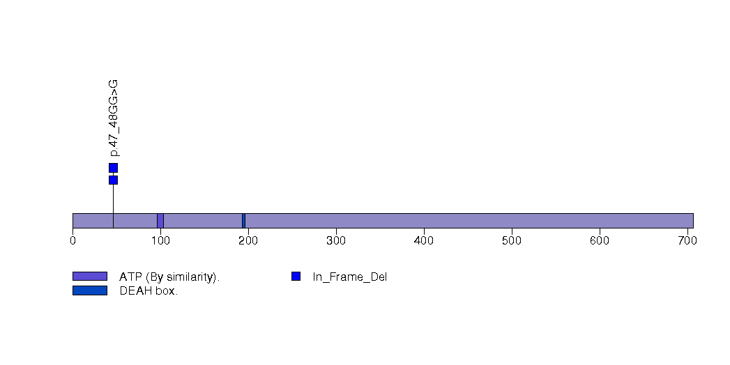
| 8 | DHX33 | DEAH (Asp-Glu-Ala-His) box polypeptide 33 | 2170 | 197 | 0 | 0 | 0 | 0 | 0 | 2 | 2 | 2 | 1 | 0.00029 | 0.01 | 0.73 | 4e-05 | 0.091 |
| 9 | PLEKHG4B | pleckstrin homology domain containing, family G (with RhoGef domain) member 4B | 3886 | 128 | 0 | 0 | 1 | 1 | 0 | 1 | 3 | 3 | 3 | 8.9e-06 | 1 | 0.38 | 0.000054 | 0.1 |
| 10 | UNC93B1 | unc-93 homolog B1 (C. elegans) | 1835 | 6 | 0 | 0 | 5 | 0 | 0 | 0 | 5 | 5 | 2 | 0.00041 | 0.0042 | 1 | 0.000055 | 0.1 |
| 11 | FNBP4 | formin binding protein 4 | 3118 | 26 | 0 | 0 | 0 | 0 | 0 | 2 | 2 | 2 | 1 | 0.00083 | 0.01 | 0.12 | 0.00011 | 0.18 |
| 12 | MAML2 | mastermind-like 2 (Drosophila) | 3487 | 279 | 0 | 0 | 0 | 0 | 0 | 2 | 2 | 2 | 1 | 0.0015 | 0.01 | 0.92 | 0.00018 | 0.28 |
| 13 | MUC21 | mucin 21, cell surface associated | 1709 | 85 | 0 | 1 | 2 | 0 | 0 | 0 | 2 | 2 | 1 | 0.0038 | 0.01 | 0.98 | 0.00042 | 0.6 |
| 14 | JPH3 | junctophilin 3 | 2263 | 298 | 0 | 0 | 2 | 0 | 0 | 0 | 2 | 2 | 1 | 0.0026 | 0.017 | 0.99 | 0.00048 | 0.63 |
| 15 | TMEM63B | transmembrane protein 63B | 2591 | 111 | 0 | 0 | 1 | 0 | 0 | 1 | 2 | 2 | 2 | 0.0067 | 1 | 0.01 | 0.00097 | 1 |
| 16 | MYH14 | myosin, heavy chain 14 | 6279 | 195 | 0 | 1 | 1 | 0 | 2 | 0 | 3 | 3 | 3 | 0.00011 | 1 | 0.67 | 0.0011 | 1 |
| 17 | PHF10 | PHD finger protein 10 | 1545 | 6 | 0 | 0 | 1 | 0 | 0 | 1 | 2 | 2 | 2 | 0.00081 | 1 | 0.12 | 0.0014 | 1 |
| 18 | GAGE13 | G antigen 13 | 374 | 5 | 0 | 0 | 0 | 0 | 0 | 1 | 1 | 1 | 1 | 0.0015 | NaN | NaN | 0.0015 | 1 |
| 19 | NCAN | neurocan | 4022 | 28 | 0 | 0 | 0 | 0 | 1 | 0 | 1 | 1 | 1 | 0.0019 | NaN | NaN | 0.0019 | 1 |
| 20 | ATP1A2 | ATPase, Na+/K+ transporting, alpha 2 (+) polypeptide | 3151 | 16 | 0 | 0 | 1 | 0 | 0 | 1 | 2 | 2 | 2 | 0.0093 | 1 | 0.021 | 0.0021 | 1 |
| 21 | WSB2 | WD repeat and SOCS box-containing 2 | 1249 | 211 | 0 | 0 | 0 | 0 | 1 | 0 | 1 | 1 | 1 | 0.0022 | NaN | NaN | 0.0022 | 1 |
| 22 | CD276 | CD276 molecule | 1641 | 53 | 0 | 0 | 0 | 1 | 0 | 0 | 1 | 1 | 1 | 0.0025 | NaN | NaN | 0.0025 | 1 |
| 23 | BACH1 | BTB and CNC homology 1, basic leucine zipper transcription factor 1 | 2227 | 86 | 0 | 0 | 8 | 1 | 0 | 0 | 9 | 1 | 9 | 0.081 | 1 | 0.00095 | 0.0026 | 1 |
| 24 | ESYT3 | extended synaptotagmin-like protein 3 | 2749 | 112 | 0 | 0 | 0 | 1 | 0 | 0 | 1 | 1 | 1 | 0.0027 | NaN | NaN | 0.0027 | 1 |
| 25 | LUZP1 | leucine zipper protein 1 | 3235 | 38 | 0 | 0 | 1 | 1 | 0 | 0 | 2 | 2 | 2 | 0.00062 | 1 | 0.47 | 0.003 | 1 |
| 26 | ALOX12 | arachidonate 12-lipoxygenase | 2046 | 64 | 0 | 0 | 0 | 1 | 0 | 0 | 1 | 1 | 1 | 0.0034 | NaN | NaN | 0.0034 | 1 |
| 27 | CYLD | cylindromatosis (turban tumor syndrome) | 2935 | 99 | 0 | 0 | 1 | 1 | 0 | 0 | 2 | 2 | 2 | 0.00042 | 1 | 0.28 | 0.0037 | 1 |
| 28 | ZNF658 | zinc finger protein 658 | 3196 | 32 | 0 | 0 | 2 | 0 | 0 | 0 | 2 | 2 | 1 | 0.045 | 0.01 | 0.38 | 0.0039 | 1 |
| 29 | HMX3 | H6 family homeobox 3 | 1077 | 62 | 0 | 0 | 0 | 0 | 0 | 1 | 1 | 1 | 1 | 0.004 | NaN | NaN | 0.004 | 1 |
| 30 | ALPK3 | alpha-kinase 3 | 5776 | 95 | 0 | 0 | 0 | 1 | 0 | 0 | 1 | 1 | 1 | 0.0042 | NaN | NaN | 0.0042 | 1 |
| 31 | L3MBTL3 | l(3)mbt-like 3 (Drosophila) | 2427 | 253 | 0 | 0 | 1 | 1 | 1 | 0 | 3 | 3 | 3 | 0.00055 | 1 | 0.83 | 0.0047 | 1 |
| 32 | EVI5L | ecotropic viral integration site 5-like | 2496 | 156 | 0 | 0 | 2 | 0 | 0 | 0 | 2 | 2 | 2 | 0.00056 | 1 | 0.8 | 0.0047 | 1 |
| 33 | COX8A | cytochrome c oxidase subunit 8A (ubiquitous) | 216 | 29 | 0 | 0 | 1 | 0 | 0 | 0 | 1 | 1 | 1 | 0.005 | NaN | NaN | 0.005 | 1 |
| 34 | FOXE3 | forkhead box E3 | 960 | 17 | 0 | 0 | 0 | 0 | 0 | 1 | 1 | 1 | 1 | 0.0052 | NaN | NaN | 0.0052 | 1 |
| 35 | DGKZ | diacylglycerol kinase, zeta 104kDa | 3923 | 29 | 0 | 0 | 0 | 0 | 0 | 1 | 1 | 1 | 1 | 0.0053 | NaN | NaN | 0.0053 | 1 |
Figure S1. This figure depicts the distribution of mutations and mutation types across the GTF2I significant gene.
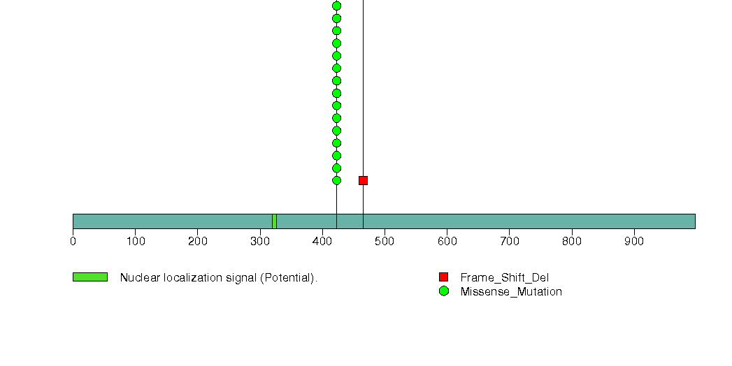
Figure S2. This figure depicts the distribution of mutations and mutation types across the HRAS significant gene.
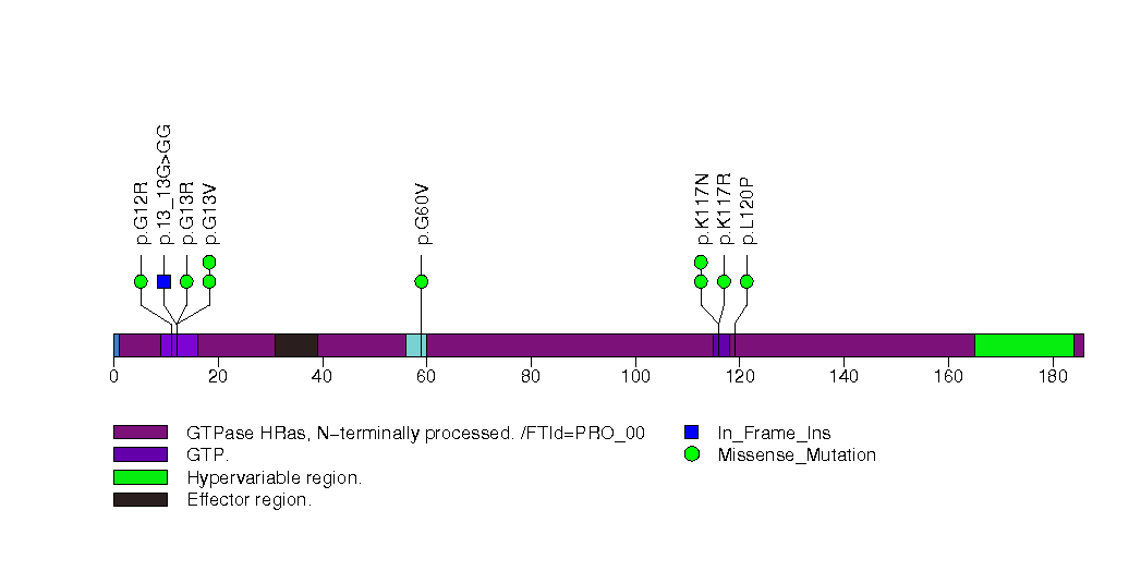
Figure S3. This figure depicts the distribution of mutations and mutation types across the CAPNS1 significant gene.
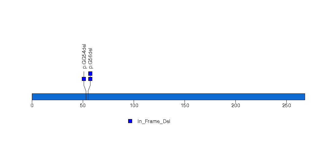
Figure S4. This figure depicts the distribution of mutations and mutation types across the TP53 significant gene.
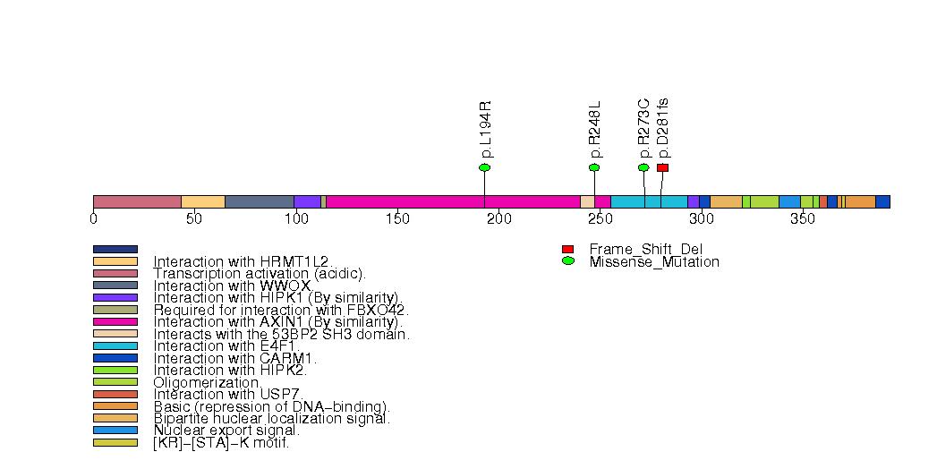
Figure S5. This figure depicts the distribution of mutations and mutation types across the ATRN significant gene.
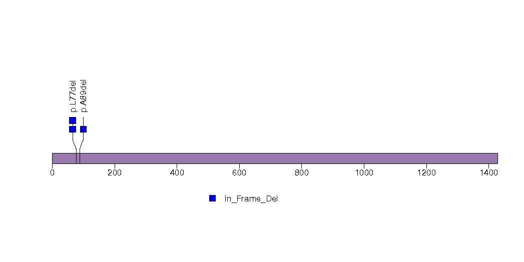
Figure S6. This figure depicts the distribution of mutations and mutation types across the FOXD1 significant gene.
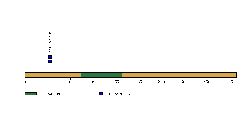
Figure S7. This figure depicts the distribution of mutations and mutation types across the NRAS significant gene.
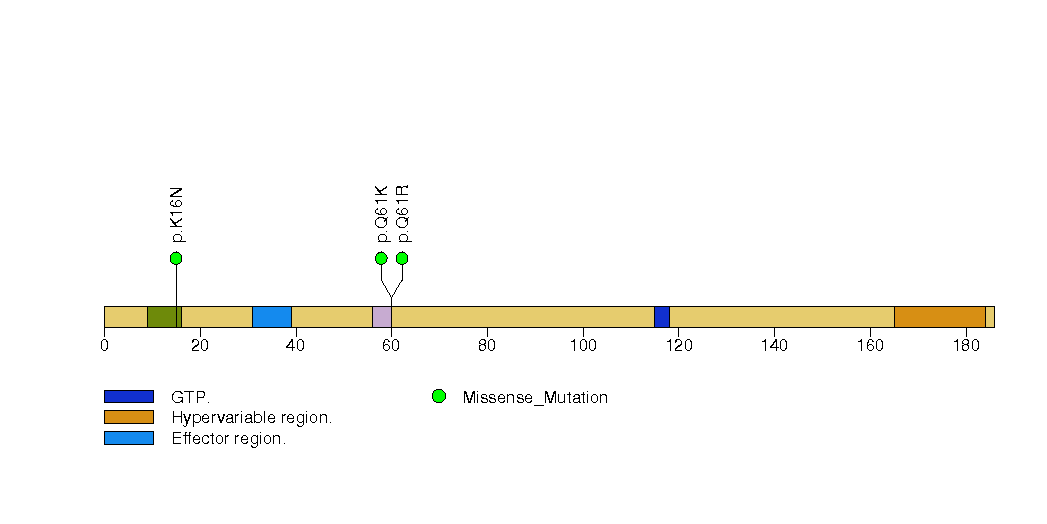
Figure S8. This figure depicts the distribution of mutations and mutation types across the DHX33 significant gene.
MutSig and its evolving algorithms have existed since the youth of clinical sequencing, with early versions used in multiple publications. [1][2][3]
"Three significance metrics [are] calculated for each gene, using the […] methods MutSigCV [4], MutSigCL, and MutSigFN [5]. These measure the significance of mutation burden, clustering, and functional impact, respectively […]. MutSigCV determines the P value for observing the given quantity of non-silent mutations in the gene, given the background model determined by silent (and noncoding) mutations in the same gene and the neighbouring genes of covariate space that form its 'bagel'. […] MutSigCL and MutSigFN measure the significance of the positional clustering of the mutations observed, as well as the significance of the tendency for mutations to occur at positions that are highly evolutionarily conserved (using conservation as a proxy for probably functional impact). MutSigCL and MutSigFN are permutation-based methods and their P values are calculated as follows: The observed nonsilent coding mutations in the gene are permuted T times (to simulate the null hypothesis, T = 108 for the most significant genes), randomly reassigning their positions, but preserving their mutational 'category', as determined by local sequence context. We [use] the following context categories: transitions at CpG dinucleotides, transitions at other C-G base pairs, transversions at C-G base pairs, mutations at A-T base pairs, and indels. Indels are unconstrained in terms of where they can move to in the permutations. For each of the random permutations, two scores are calculated: SCL and SFN, measuring the amount of clustering and function impact (measured by conservation) respectively. SCL is defined to be the fraction of mutations occurring in hotspots. A hotspot is defined as a 3-base-pair region of the gene containing many mutations: at least 2, and at least 2% of the total mutations. SFN is defined to be the mean of the base-pair-level conservation values for the position of each non-silent mutation […]. To determine a PCL, the P value for the observed degree of positional clustering, the observed value of SCL (computed for the mutations actually observed), [is] compared to the distribution of SCL obtained from the random permutations, and the P value [is] defined to be the fraction of random permutations in which SCL [is] at least as large as the observed SCL. The P value for the conservation of the mutated positions, PFN, [is] computed analogously." [6]
In addition to the links below, the full results of the analysis summarized in this report can also be downloaded programmatically using firehose_get, or interactively from either the Broad GDAC website or TCGA Data Coordination Center Portal.