Skin Cutaneous Melanoma: Correlation between molecular cancer subtypes and selected clinical features

Maintained by TCGA GDAC Team (Broad Institute/MD Anderson Cancer Center/Harvard Medical School)

Overview

Introduction

This pipeline computes the correlation between cancer subtypes identified by different molecular patterns and selected clinical features.

Summary

Testing the association between subtypes identified by 6 different clustering approaches and 3 clinical features across 144 patients, one significant finding detected with P value < 0.05 and Q value < 0.25.

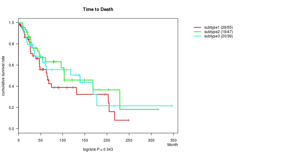
3 subtypes identified in current cancer cohort by 'CN CNMF'. These subtypes do not correlate to any clinical features.
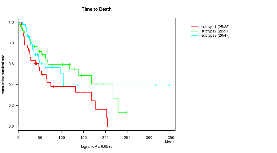
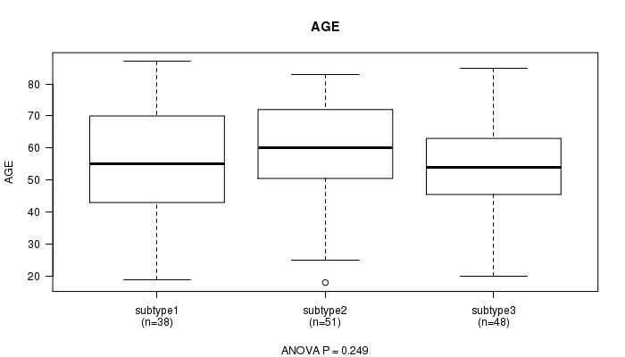
3 subtypes identified in current cancer cohort by 'METHLYATION CNMF'. These subtypes do not correlate to any clinical features.
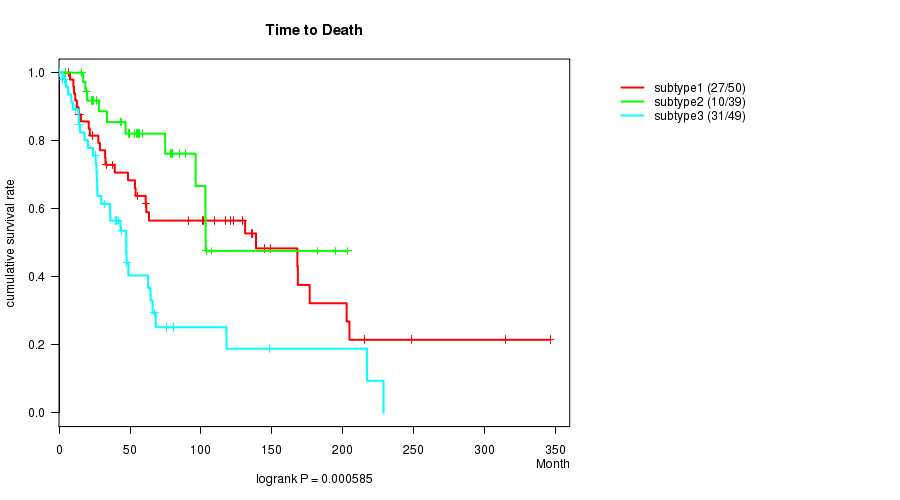
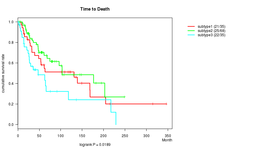
CNMF clustering analysis on sequencing-based mRNA expression data identified 3 subtypes that correlate to 'Time to Death'.
Consensus hierarchical clustering analysis on sequencing-based mRNA expression data identified 3 subtypes that do not correlate to any clinical features.
CNMF clustering analysis on sequencing-based miR expression data identified 4 subtypes that do not correlate to any clinical features.
Consensus hierarchical clustering analysis on sequencing-based miR expression data identified 3 subtypes that do not correlate to any clinical features.

Results

Overview of the results

Table 1. Get Full Table Overview of the association between subtypes identified by 6 different clustering approaches and 3 clinical features. Shown in the table are P values (Q values). Thresholded by P value < 0.05 and Q value < 0.25, one significant finding detected.


Clinical Features	Time to Death	AGE	GENDER
Statistical Tests	logrank test	ANOVA	Fisher's exact test
CN CNMF	0.343 (1.00)	0.304 (1.00)	0.975 (1.00)
METHLYATION CNMF	0.0535 (0.855)	0.249 (1.00)	0.172 (1.00)
RNAseq CNMF subtypes	0.000585 (0.0105)	0.0536 (0.855)	0.408 (1.00)
RNAseq cHierClus subtypes	0.0189 (0.321)	0.0729 (1.00)	0.467 (1.00)
MIRseq CNMF subtypes	0.135 (1.00)	0.37 (1.00)	0.609 (1.00)
MIRseq cHierClus subtypes	0.197 (1.00)	0.398 (1.00)	0.861 (1.00)

Clustering Approach #1: 'CN CNMF'

Table S1. Get Full Table Description of clustering approach #1: 'CN CNMF'

Cluster Labels	1	2	3
Number of samples	56	47	41

'CN CNMF' versus 'Time to Death'

P value = 0.343 (logrank test), Q value = 1

Table S2. Clustering Approach #1: 'CN CNMF' versus Clinical Feature #1: 'Time to Death'

	nPatients	nDeath	Duration Range (Median), Month
ALL	141	68	0.2 - 346.0 (47.5)
subtype1	55	29	0.2 - 248.6 (41.6)
subtype2	47	19	4.2 - 314.5 (46.8)
subtype3	39	20	6.4 - 346.0 (58.8)

Figure S1. Get High-res Image Clustering Approach #1: 'CN CNMF' versus Clinical Feature #1: 'Time to Death'

'CN CNMF' versus 'AGE'

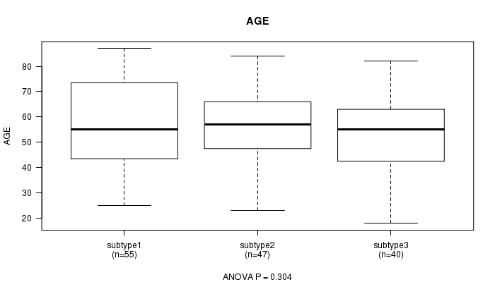
P value = 0.304 (ANOVA), Q value = 1

Table S3. Clustering Approach #1: 'CN CNMF' versus Clinical Feature #2: 'AGE'

	nPatients	Mean (Std.Dev)
ALL	142	56.0 (16.2)
subtype1	55	57.5 (18.0)
subtype2	47	57.1 (13.7)
subtype3	40	52.6 (16.3)

Figure S2. Get High-res Image Clustering Approach #1: 'CN CNMF' versus Clinical Feature #2: 'AGE'

'CN CNMF' versus 'GENDER'

P value = 0.975 (Fisher's exact test), Q value = 1

Table S4. Clustering Approach #1: 'CN CNMF' versus Clinical Feature #3: 'GENDER'

nPatients	FEMALE	MALE
ALL	51	93
subtype1	20	36
subtype2	16	31
subtype3	15	26

Figure S3. Get High-res Image Clustering Approach #1: 'CN CNMF' versus Clinical Feature #3: 'GENDER'

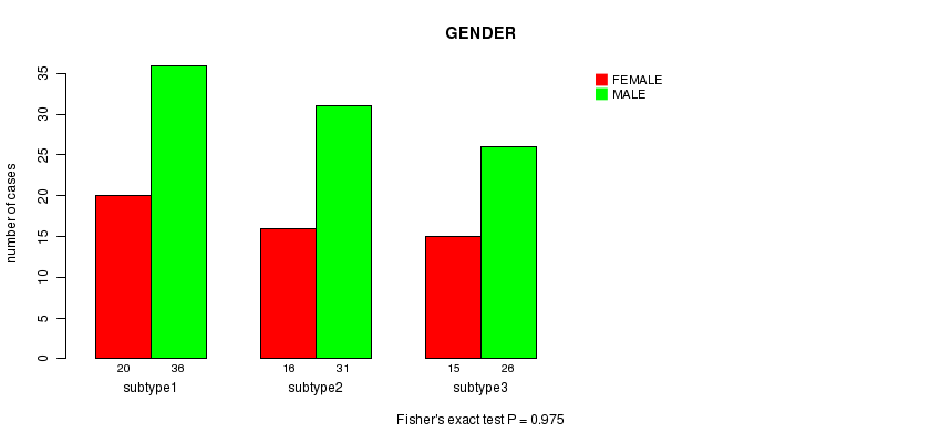
Clustering Approach #2: 'METHLYATION CNMF'

Table S5. Get Full Table Description of clustering approach #2: 'METHLYATION CNMF'

Cluster Labels	1	2	3
Number of samples	38	53	48

'METHLYATION CNMF' versus 'Time to Death'

P value = 0.0535 (logrank test), Q value = 0.86

Table S6. Clustering Approach #2: 'METHLYATION CNMF' versus Clinical Feature #1: 'Time to Death'

	nPatients	nDeath	Duration Range (Median), Month
ALL	136	67	0.2 - 346.0 (47.5)
subtype1	38	25	0.2 - 204.6 (39.9)
subtype2	51	22	2.6 - 248.6 (53.9)
subtype3	47	20	2.7 - 346.0 (47.3)

Figure S4. Get High-res Image Clustering Approach #2: 'METHLYATION CNMF' versus Clinical Feature #1: 'Time to Death'

'METHLYATION CNMF' versus 'AGE'

P value = 0.249 (ANOVA), Q value = 1

Table S7. Clustering Approach #2: 'METHLYATION CNMF' versus Clinical Feature #2: 'AGE'

	nPatients	Mean (Std.Dev)
ALL	137	56.5 (16.2)
subtype1	38	55.3 (17.1)
subtype2	51	59.4 (16.6)
subtype3	48	54.2 (14.7)

Figure S5. Get High-res Image Clustering Approach #2: 'METHLYATION CNMF' versus Clinical Feature #2: 'AGE'

'METHLYATION CNMF' versus 'GENDER'

P value = 0.172 (Fisher's exact test), Q value = 1

Table S8. Clustering Approach #2: 'METHLYATION CNMF' versus Clinical Feature #3: 'GENDER'

nPatients	FEMALE	MALE
ALL	51	88
subtype1	14	24
subtype2	24	29
subtype3	13	35

Figure S6. Get High-res Image Clustering Approach #2: 'METHLYATION CNMF' versus Clinical Feature #3: 'GENDER'

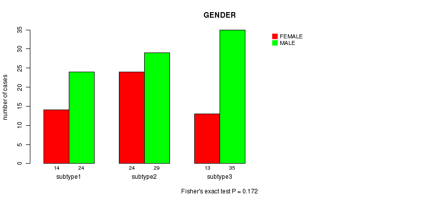
Clustering Approach #3: 'RNAseq CNMF subtypes'

Table S9. Get Full Table Description of clustering approach #3: 'RNAseq CNMF subtypes'

Cluster Labels	1	2	3
Number of samples	51	40	50

'RNAseq CNMF subtypes' versus 'Time to Death'

P value = 0.000585 (logrank test), Q value = 0.011

Table S10. Clustering Approach #3: 'RNAseq CNMF subtypes' versus Clinical Feature #1: 'Time to Death'

	nPatients	nDeath	Duration Range (Median), Month
ALL	138	68	0.2 - 346.0 (47.5)
subtype1	50	27	6.4 - 346.0 (61.3)
subtype2	39	10	4.2 - 203.0 (53.3)
subtype3	49	31	0.2 - 228.6 (35.9)

Figure S7. Get High-res Image Clustering Approach #3: 'RNAseq CNMF subtypes' versus Clinical Feature #1: 'Time to Death'

'RNAseq CNMF subtypes' versus 'AGE'

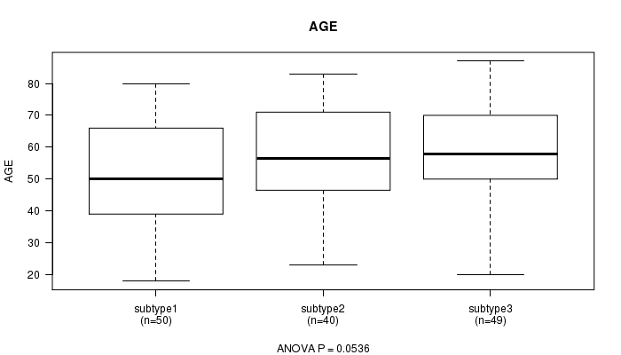
P value = 0.0536 (ANOVA), Q value = 0.86

Table S11. Clustering Approach #3: 'RNAseq CNMF subtypes' versus Clinical Feature #2: 'AGE'

	nPatients	Mean (Std.Dev)
ALL	139	56.1 (16.3)
subtype1	50	51.7 (16.7)
subtype2	40	57.8 (15.8)
subtype3	49	59.1 (15.7)

Figure S8. Get High-res Image Clustering Approach #3: 'RNAseq CNMF subtypes' versus Clinical Feature #2: 'AGE'

'RNAseq CNMF subtypes' versus 'GENDER'

P value = 0.408 (Fisher's exact test), Q value = 1

Table S12. Clustering Approach #3: 'RNAseq CNMF subtypes' versus Clinical Feature #3: 'GENDER'

nPatients	FEMALE	MALE
ALL	50	91
subtype1	21	30
subtype2	11	29
subtype3	18	32

Figure S9. Get High-res Image Clustering Approach #3: 'RNAseq CNMF subtypes' versus Clinical Feature #3: 'GENDER'

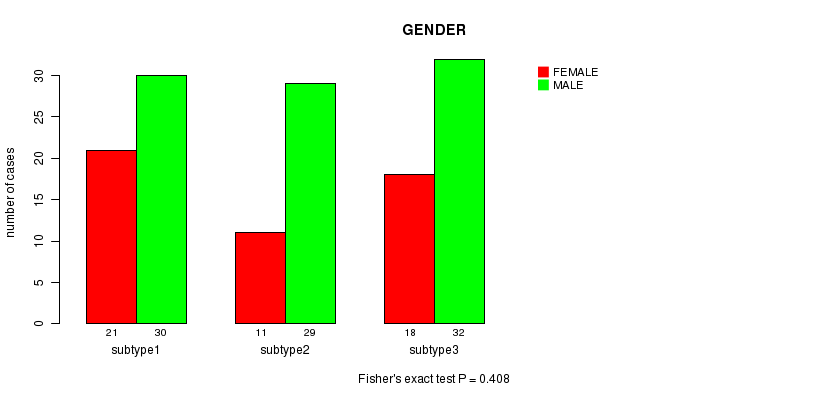
Clustering Approach #4: 'RNAseq cHierClus subtypes'

Table S13. Get Full Table Description of clustering approach #4: 'RNAseq cHierClus subtypes'

Cluster Labels	1	2	3
Number of samples	36	69	36

'RNAseq cHierClus subtypes' versus 'Time to Death'

P value = 0.0189 (logrank test), Q value = 0.32

Table S14. Clustering Approach #4: 'RNAseq cHierClus subtypes' versus Clinical Feature #1: 'Time to Death'

	nPatients	nDeath	Duration Range (Median), Month
ALL	138	68	0.2 - 346.0 (47.5)
subtype1	35	21	7.8 - 346.0 (61.2)
subtype2	68	25	2.7 - 248.6 (49.2)
subtype3	35	22	0.2 - 228.6 (33.2)

Figure S10. Get High-res Image Clustering Approach #4: 'RNAseq cHierClus subtypes' versus Clinical Feature #1: 'Time to Death'

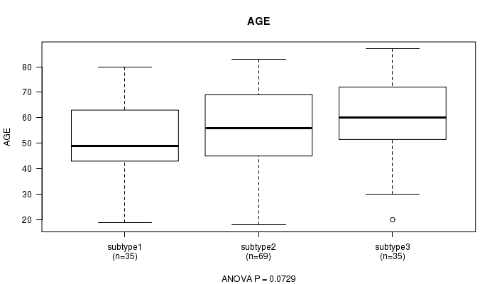
'RNAseq cHierClus subtypes' versus 'AGE'

P value = 0.0729 (ANOVA), Q value = 1

Table S15. Clustering Approach #4: 'RNAseq cHierClus subtypes' versus Clinical Feature #2: 'AGE'

	nPatients	Mean (Std.Dev)
ALL	139	56.1 (16.3)
subtype1	35	51.5 (15.5)
subtype2	69	56.1 (16.3)
subtype3	35	60.5 (16.5)

Figure S11. Get High-res Image Clustering Approach #4: 'RNAseq cHierClus subtypes' versus Clinical Feature #2: 'AGE'

'RNAseq cHierClus subtypes' versus 'GENDER'

P value = 0.467 (Fisher's exact test), Q value = 1

Table S16. Clustering Approach #4: 'RNAseq cHierClus subtypes' versus Clinical Feature #3: 'GENDER'

nPatients	FEMALE	MALE
ALL	50	91
subtype1	15	21
subtype2	21	48
subtype3	14	22

Figure S12. Get High-res Image Clustering Approach #4: 'RNAseq cHierClus subtypes' versus Clinical Feature #3: 'GENDER'

Clustering Approach #5: 'MIRseq CNMF subtypes'

Table S17. Get Full Table Description of clustering approach #5: 'MIRseq CNMF subtypes'

Cluster Labels	1	2	3	4	5
Number of samples	31	50	31	22	2

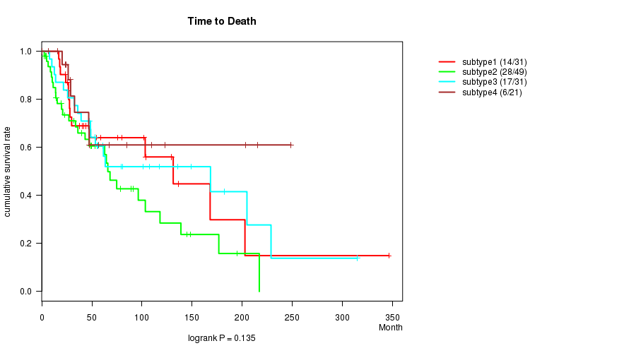
'MIRseq CNMF subtypes' versus 'Time to Death'

P value = 0.135 (logrank test), Q value = 1

Table S18. Clustering Approach #5: 'MIRseq CNMF subtypes' versus Clinical Feature #1: 'Time to Death'

	nPatients	nDeath	Duration Range (Median), Month
ALL	132	65	0.2 - 346.0 (47.5)
subtype1	31	14	17.0 - 346.0 (44.0)
subtype2	49	28	2.6 - 216.9 (43.2)
subtype3	31	17	7.8 - 314.5 (55.9)
subtype4	21	6	0.2 - 248.6 (46.8)

Figure S13. Get High-res Image Clustering Approach #5: 'MIRseq CNMF subtypes' versus Clinical Feature #1: 'Time to Death'

'MIRseq CNMF subtypes' versus 'AGE'

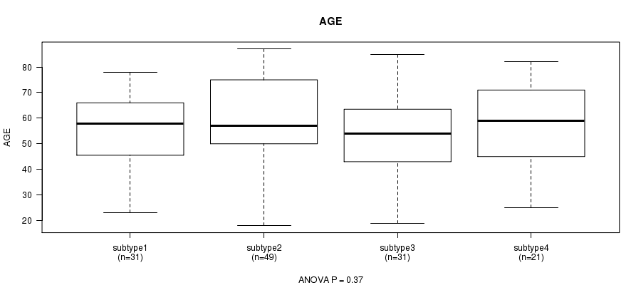
P value = 0.37 (ANOVA), Q value = 1

Table S19. Clustering Approach #5: 'MIRseq CNMF subtypes' versus Clinical Feature #2: 'AGE'

	nPatients	Mean (Std.Dev)
ALL	132	56.2 (16.2)
subtype1	31	54.5 (13.7)
subtype2	49	59.0 (16.6)
subtype3	31	52.8 (17.3)
subtype4	21	56.8 (17.0)

Figure S14. Get High-res Image Clustering Approach #5: 'MIRseq CNMF subtypes' versus Clinical Feature #2: 'AGE'

'MIRseq CNMF subtypes' versus 'GENDER'

P value = 0.609 (Fisher's exact test), Q value = 1

Table S20. Clustering Approach #5: 'MIRseq CNMF subtypes' versus Clinical Feature #3: 'GENDER'

nPatients	FEMALE	MALE
ALL	47	87
subtype1	13	18
subtype2	18	32
subtype3	8	23
subtype4	8	14

Figure S15. Get High-res Image Clustering Approach #5: 'MIRseq CNMF subtypes' versus Clinical Feature #3: 'GENDER'

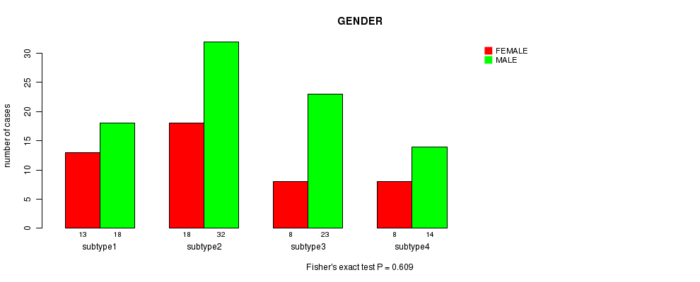
Clustering Approach #6: 'MIRseq cHierClus subtypes'

Table S21. Get Full Table Description of clustering approach #6: 'MIRseq cHierClus subtypes'

Cluster Labels	1	2	3
Number of samples	16	89	31

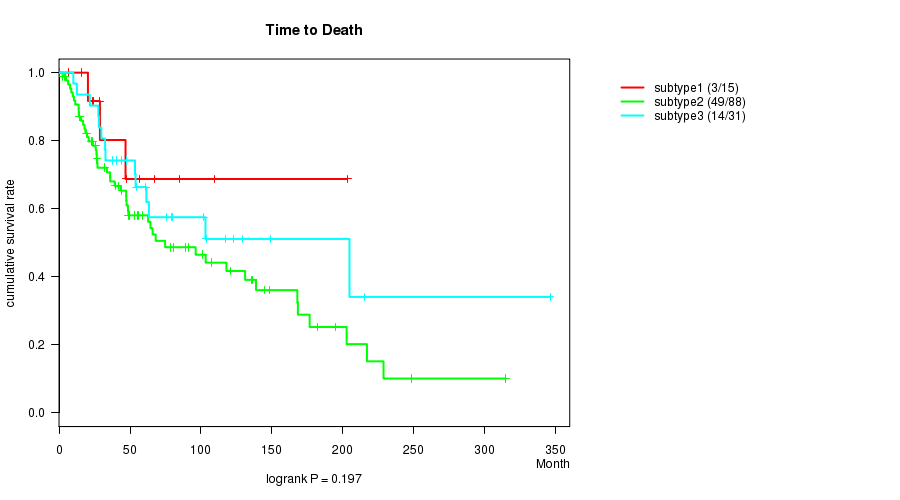
'MIRseq cHierClus subtypes' versus 'Time to Death'

P value = 0.197 (logrank test), Q value = 1

Table S22. Clustering Approach #6: 'MIRseq cHierClus subtypes' versus Clinical Feature #1: 'Time to Death'

	nPatients	nDeath	Duration Range (Median), Month
ALL	134	66	0.2 - 346.0 (47.7)
subtype1	15	3	0.2 - 203.0 (28.8)
subtype2	88	49	2.6 - 314.5 (47.3)
subtype3	31	14	10.1 - 346.0 (61.2)

Figure S16. Get High-res Image Clustering Approach #6: 'MIRseq cHierClus subtypes' versus Clinical Feature #1: 'Time to Death'

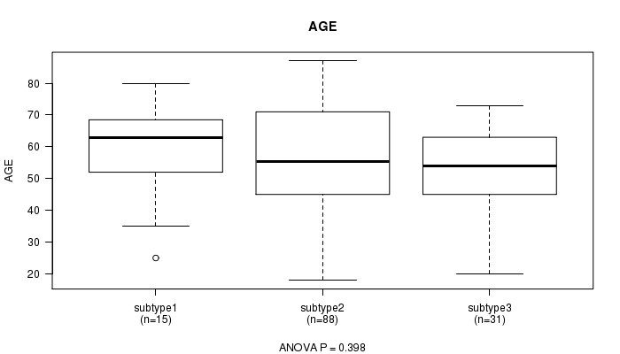
'MIRseq cHierClus subtypes' versus 'AGE'

P value = 0.398 (ANOVA), Q value = 1

Table S23. Clustering Approach #6: 'MIRseq cHierClus subtypes' versus Clinical Feature #2: 'AGE'

	nPatients	Mean (Std.Dev)
ALL	134	56.1 (16.1)
subtype1	15	58.5 (15.8)
subtype2	88	56.9 (16.9)
subtype3	31	52.8 (13.7)

Figure S17. Get High-res Image Clustering Approach #6: 'MIRseq cHierClus subtypes' versus Clinical Feature #2: 'AGE'

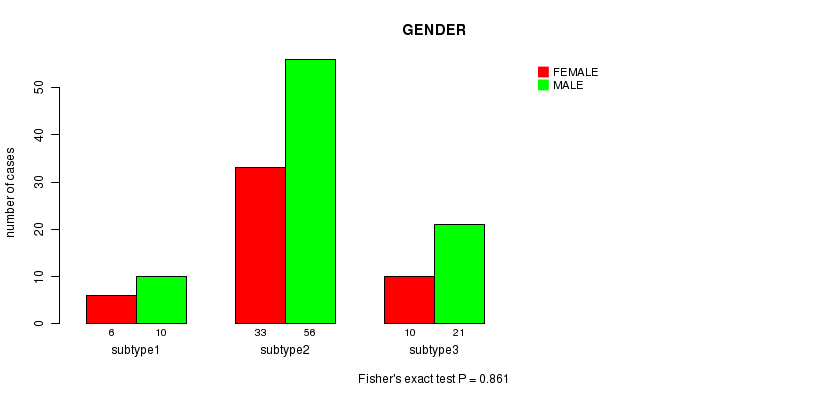
'MIRseq cHierClus subtypes' versus 'GENDER'

P value = 0.861 (Fisher's exact test), Q value = 1

Table S24. Clustering Approach #6: 'MIRseq cHierClus subtypes' versus Clinical Feature #3: 'GENDER'

nPatients	FEMALE	MALE
ALL	49	87
subtype1	6	10
subtype2	33	56
subtype3	10	21

Figure S18. Get High-res Image Clustering Approach #6: 'MIRseq cHierClus subtypes' versus Clinical Feature #3: 'GENDER'

Methods & Data

Input

Cluster data file = SKCM-TM.mergedcluster.txt
Clinical data file = SKCM-TM.clin.merged.picked.txt
Number of patients = 144
Number of clustering approaches = 6
Number of selected clinical features = 3
Exclude small clusters that include fewer than K patients, K = 3

Clustering approaches

CNMF clustering

consensus non-negative matrix factorization clustering approach (Brunet et al. 2004)

Consensus hierarchical clustering

Resampling-based clustering method (Monti et al. 2003)

Survival analysis

For survival clinical features, the Kaplan-Meier survival curves of tumors with and without gene mutations were plotted and the statistical significance P values were estimated by logrank test (Bland and Altman 2004) using the 'survdiff' function in R

ANOVA analysis

For continuous numerical clinical features, one-way analysis of variance (Howell 2002) was applied to compare the clinical values between tumor subtypes using 'anova' function in R

Fisher's exact test

For binary clinical features, two-tailed Fisher's exact tests (Fisher 1922) were used to estimate the P values using the 'fisher.test' function in R

Q value calculation

For multiple hypothesis correction, Q value is the False Discovery Rate (FDR) analogue of the P value (Benjamini and Hochberg 1995), defined as the minimum FDR at which the test may be called significant. We used the 'Benjamini and Hochberg' method of 'p.adjust' function in R to convert P values into Q values.

Download Results

This is an experimental feature. The full results of the analysis summarized in this report can be downloaded from the TCGA Data Coordination Center.

References

[1] Brunet et al., Metagenes and molecular pattern discovery using matrix factorization, PNAS 101(12):4164-9 (2004)

[2] Monti et al., Consensus Clustering: A Resampling-Based Method for Class Discovery and Visualization of Gene Expression Microarray Data, Machine Learning 52(1):91-118 (2003)

[3] Bland and Altman, Statistics notes: The logrank test, BMJ 328(7447):1073 (2004)

[4] Howell, D, Statistical Methods for Psychology. (5th ed.), Duxbury Press:324-5 (2002)

[5] Fisher, R.A., On the interpretation of chi-square from contingency tables, and the calculation of P, Journal of the Royal Statistical Society 85(1):87-94 (1922)

[6] Benjamini and Hochberg, Controlling the false discovery rate: a practical and powerful approach to multiple testing, Journal of the Royal Statistical Society Series B 59:289-300 (1995)

Made with Nozzle