This report serves to describe the mutational landscape and properties of a given cohort, as well as rank genes and genesets according to mutational significance. MutSig 2CV v3.1 hg38 beta was used to generate the results found in this report.
-
Working with cohort: PanCan
-
Number of patients in cohort: 417
**Please note that in this beta version for hg38 MAFs only the burden test (MutSigCV) is utilized. Beta version does not support positional or functional clustering tests (MutSigCL/MutSigFN, respectively). These tests currently only work in the hg19 compatible release.**
The input for this pipeline is an annotated .maf file describing the mutations called for each individual in the given cancer cohort, and their properties.
-
MAF used for this analysis: PanCan.final_analysis_set.maf
-
Significantly mutated genes (q ≤ 0.1): 56
Table 1. Get Full Table A breakdown of mutation rates per category discovered for this cohort.
| left | from | change | right | n | N | rate | ci_low | ci_high | relrate | autoname | name | type |
|---|---|---|---|---|---|---|---|---|---|---|---|---|
| ACGT | C | t | G | 17395 | 2167158677 | 8e-06 | 7.9e-06 | 8.1e-06 | 8.4 | ACGT[C->t]G | *CpG->T | point |
| ACGT | C | s | ACGT | 40524 | 20149175747 | 2e-06 | 2e-06 | 2e-06 | 2.1 | ACGT[C->s]ACGT | C->A | point |
| ACGT | C | t | ACT | 19556 | 17982017070 | 1.1e-06 | 1.1e-06 | 1.1e-06 | 1.1 | ACGT[C->t]ACT | *Cp(A/C/T)->T | point |
| ACGT | C | f | ACGT | 10146 | 20149175747 | 5e-07 | 4.9e-07 | 5.1e-07 | 0.53 | ACGT[C->f]ACGT | C->G | point |
| ACGT | A | tfs | ACGT | 25569 | 58467726840 | 4.4e-07 | 4.3e-07 | 4.4e-07 | 0.46 | ACGT[A->tfs]ACGT | A->mut | point |
The mutation spectrum is depicted in the lego plots below in which the 96 possible mutation types are subdivided into six large blocks, color-coded to reflect the base substitution type. Each large block is further subdivided into the 16 possible pairs of 5' and 3' neighbors, as listed in the 4x4 trinucleotide context legend. The height of each block corresponds to the mutation frequency for that kind of mutation (counts of mutations normalized by the base coverage in a given bin). The shape of the spectrum is a signature for dominant mutational mechanisms in different tumor types.
Figure 1. Get High-res Image SNV Mutation rate lego plot for entire cohort. Each bin is normalized by base coverage for that bin. Colors represent the six SNV types on the upper right. The three-base context for each mutation is labeled in the 4x4 legend on the lower right. The fractional breakdown of SNV counts is shown in the pie chart on the upper left. If this figure is blank, not enough information was provided in the MAF to generate it.
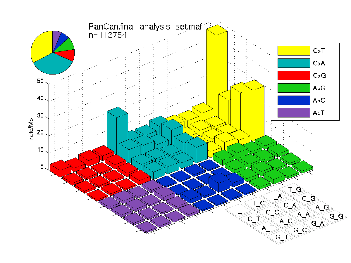
Figure 2. Get High-res Image SNV Mutation rate lego plots for 4 slices of mutation allele fraction (0<=AF<0.1, 0.1<=AF<0.25, 0.25<=AF<0.5, & 0.5<=AF) . The color code and three-base context legends are the same as the previous figure. If this figure is blank, not enough information was provided in the MAF to generate it.
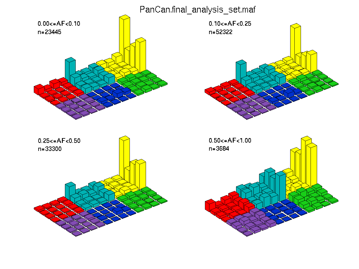
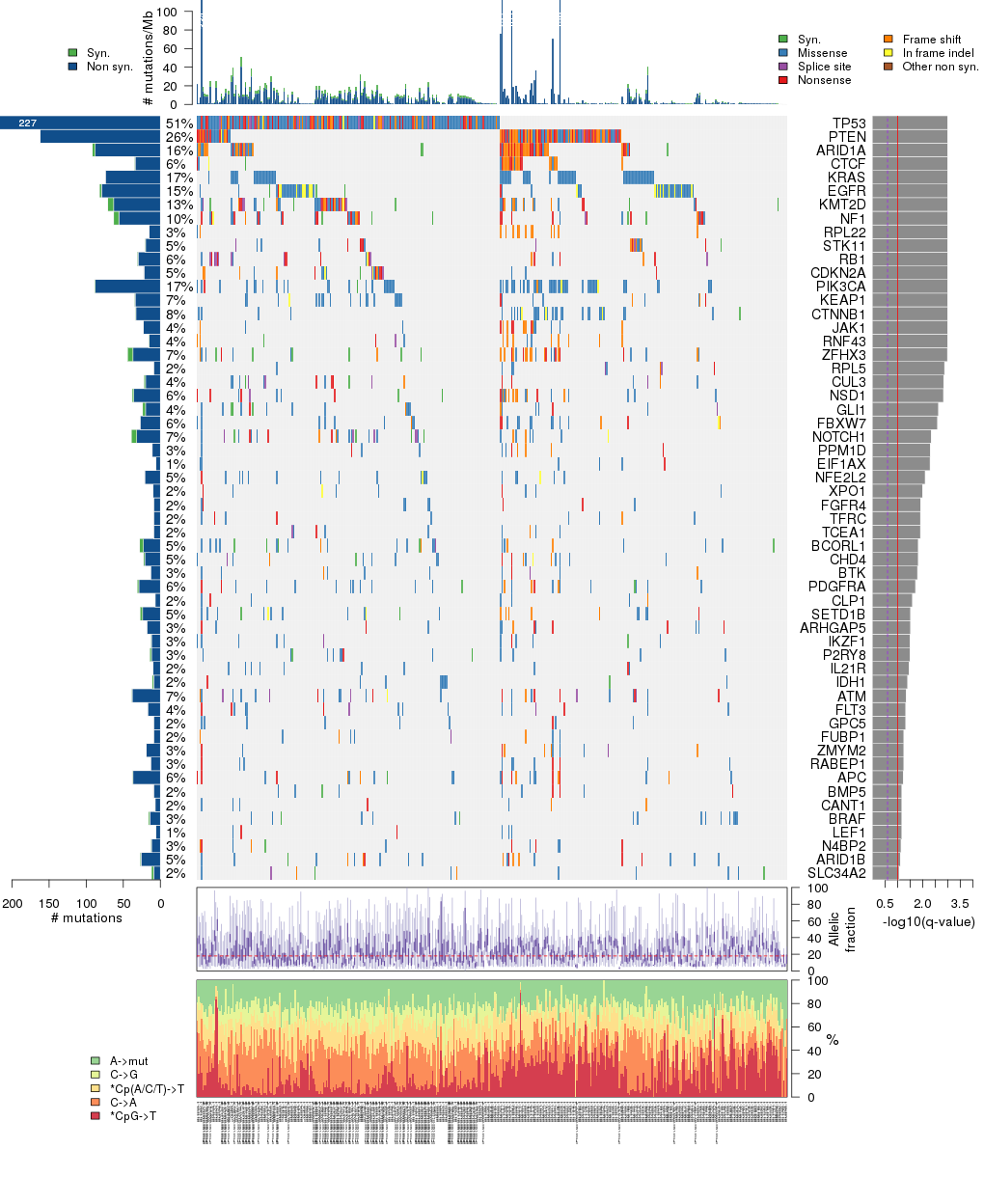
Figure 3. Get High-res Image The matrix in the center of the figure represents individual mutations in patient samples, color-coded by type of mutation, for the significantly mutated genes. The rate of synonymous and non-synonymous mutations is displayed at the top of the matrix. The barplot on the left of the matrix shows the number of mutations in each gene. The percentages represent the fraction of tumors with at least one mutation in the specified gene. The barplot to the right of the matrix displays the q-values for the most significantly mutated genes. The purple boxplots below the matrix (only displayed if required columns are present in the provided MAF) represent the distributions of allelic fractions observed in each sample. The plot at the bottom represents the base substitution distribution of individual samples, using the same categories that were used to calculate significance.
Column Descriptions:
-
codelen = the gene's coding length
-
nncd = number of noncoding mutations in this gene across the cohort
-
nsil = number of silent mutations in this gene across the cohort
-
nmis = number of missense mutations in this gene across the cohort
-
nstp = number of readthrough mutations in this gene across the cohort
-
nspl = number of splice site mutations in this gene across the cohort
-
nind = number of indels in this gene across the cohort
-
nnon = number of (nonsilent) mutations in this gene across the cohort
-
npat = number of patients (individuals) with at least one nonsilent mutation
-
nsite = number of unique sites having a non-silent mutation
-
Abundance (pCV) = Probability that the gene's overall nonsilent mutation rate exceeds its inferred background mutation rate (BMR), which is computed based on the gene's own silent mutation rate plus silent mutation rates of genes with similar covariates. BMR calculations are normalized with respect to patient-specific and sequence context-specific mutation rates.
-
Clustering (pCL) = Probability that recurrently mutated loci in this gene have more mutations than expected by chance. While pCV assesses the gene's overall mutation burden, pCL assesses the burden of specific sites within the gene. This allows MutSig to differentiate between genes with uniformly distributed mutations and genes with localized hotspots.
-
Conservation (pFN) = Probability that mutations within this gene occur disproportionately at evolutionarily conserved sites. Sites highly conserved across vertebrates are assumed to have greater functional impact than weakly conserved sites.
-
p = p-value (overall)
-
q = q-value, False Discovery Rate (Benjamini-Hochberg procedure)
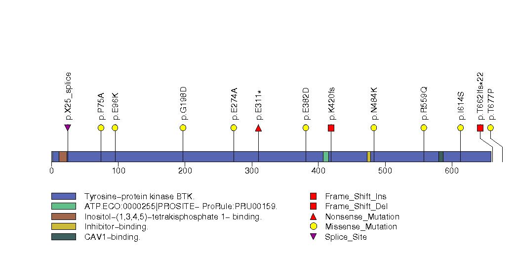
Table 2. Get Full Table A Ranked List of Significantly Mutated Genes. Number of significant genes found: 56. Number of genes displayed: 35. Click on a gene name to display its stick figure depicting the distribution of mutations and mutation types across the chosen gene (this feature may not be available for all significant genes).
| rank | gene | codelen | nnei | nncd | nsil | nmis | nstp | nspl | nind | nnon | npat | nsite | pCV | pCL | pFN | p | q |
|---|---|---|---|---|---|---|---|---|---|---|---|---|---|---|---|---|---|
| 1 | TP53 | 1613 | 47 | 0 | 0 | 152 | 34 | 12 | 29 | 227 | 214 | 138 | 1e-16 | NA | NA | 1e-16 | 2.3e-14 |
| 2 | PTEN | 1407 | 117 | 0 | 0 | 79 | 36 | 5 | 42 | 162 | 110 | 103 | 1e-16 | NA | NA | 1e-16 | 2.3e-14 |
| 3 | ARID1A | 7104 | 3 | 0 | 4 | 26 | 19 | 1 | 42 | 88 | 65 | 76 | 1e-16 | NA | NA | 1e-16 | 2.3e-14 |
| 4 | CTCF | 2352 | 1 | 0 | 1 | 9 | 8 | 0 | 17 | 34 | 26 | 28 | 1.6e-16 | NA | NA | 1.6e-16 | 2.8e-14 |
| 5 | KRAS | 832 | 12 | 0 | 0 | 74 | 0 | 0 | 0 | 74 | 72 | 9 | 1.4e-15 | NA | NA | 1.4e-15 | 1.9e-13 |
| 6 | EGFR | 4409 | 38 | 0 | 3 | 57 | 3 | 0 | 19 | 79 | 64 | 38 | 2.7e-15 | NA | NA | 2.7e-15 | 3.1e-13 |
| 7 | KMT2D | 17250 | 22 | 0 | 8 | 29 | 12 | 7 | 15 | 63 | 54 | 62 | 1.7e-14 | NA | NA | 1.7e-14 | 1.7e-12 |
| 8 | NF1 | 9208 | 36 | 0 | 7 | 26 | 21 | 3 | 6 | 56 | 40 | 54 | 9.2e-14 | NA | NA | 9.2e-14 | 8.1e-12 |
| 9 | RPL22 | 490 | 42 | 0 | 0 | 1 | 0 | 0 | 14 | 15 | 14 | 4 | 2.3e-13 | NA | NA | 2.3e-13 | 1.8e-11 |
| 10 | STK11 | 1428 | 60 | 0 | 1 | 7 | 6 | 3 | 4 | 20 | 20 | 20 | 3e-13 | NA | NA | 3e-13 | 2.1e-11 |
| 11 | RB1 | 3111 | 16 | 0 | 1 | 8 | 9 | 9 | 4 | 30 | 24 | 29 | 1.2e-11 | NA | NA | 1.2e-11 | 7.3e-10 |
| 12 | CDKN2A | 984 | 9 | 0 | 1 | 8 | 5 | 2 | 7 | 22 | 22 | 20 | 1.4e-09 | NA | NA | 1.4e-09 | 8e-08 |
| 13 | PIK3CA | 3465 | 7 | 0 | 1 | 83 | 1 | 0 | 4 | 88 | 72 | 46 | 3.3e-09 | NA | NA | 3.3e-09 | 1.8e-07 |
| 14 | KEAP1 | 1959 | 16 | 0 | 1 | 29 | 2 | 0 | 3 | 34 | 28 | 33 | 1.1e-08 | NA | NA | 1.1e-08 | 5.7e-07 |
| 15 | CTNNB1 | 2627 | 12 | 0 | 1 | 30 | 0 | 0 | 3 | 33 | 32 | 18 | 3.9e-08 | NA | NA | 3.9e-08 | 1.8e-06 |
| 16 | JAK1 | 3777 | 0 | 0 | 0 | 6 | 4 | 1 | 12 | 23 | 18 | 14 | 8.4e-08 | NA | NA | 8.4e-08 | 3.7e-06 |
| 17 | RNF43 | 2822 | 52 | 0 | 1 | 3 | 1 | 1 | 10 | 15 | 15 | 7 | 1e-07 | NA | NA | 1e-07 | 4.2e-06 |
| 18 | ZFHX3 | 11262 | 19 | 0 | 7 | 13 | 8 | 0 | 16 | 37 | 30 | 33 | 5.1e-07 | NA | NA | 5.1e-07 | 2e-05 |
| 19 | RPL5 | 999 | 92 | 0 | 0 | 5 | 1 | 2 | 1 | 9 | 9 | 9 | 8.9e-06 | NA | NA | 8.9e-06 | 0.00033 |
| 20 | CUL3 | 2535 | 37 | 0 | 2 | 9 | 5 | 4 | 2 | 20 | 18 | 19 | 0.000013 | NA | NA | 0.000013 | 0.00044 |
| 21 | NSD1 | 8493 | 4 | 0 | 2 | 21 | 6 | 1 | 8 | 36 | 26 | 34 | 0.000014 | NA | NA | 0.000014 | 0.00047 |
| 22 | GLI1 | 3496 | 37 | 0 | 4 | 15 | 2 | 1 | 2 | 20 | 18 | 20 | 0.000043 | NA | NA | 0.000043 | 0.0014 |
| 23 | FBXW7 | 2597 | 5 | 0 | 0 | 20 | 3 | 0 | 4 | 27 | 24 | 19 | 0.000053 | NA | NA | 0.000053 | 0.0016 |
| 24 | NOTCH1 | 8076 | 2 | 0 | 7 | 18 | 3 | 5 | 6 | 32 | 28 | 32 | 0.00012 | NA | NA | 0.00012 | 0.0035 |
| 25 | PPM1D | 1929 | 1 | 0 | 0 | 5 | 3 | 0 | 3 | 11 | 11 | 10 | 0.00014 | NA | NA | 0.00014 | 0.0039 |
| 26 | EIF1AX | 531 | 103 | 0 | 0 | 5 | 1 | 0 | 0 | 6 | 6 | 6 | 0.00015 | NA | NA | 0.00015 | 0.004 |
| 27 | NFE2L2 | 1968 | 4 | 0 | 0 | 18 | 1 | 0 | 2 | 21 | 20 | 14 | 0.00027 | NA | NA | 0.00027 | 0.0069 |
| 28 | XPO1 | 3528 | 14 | 0 | 0 | 7 | 2 | 0 | 1 | 10 | 9 | 9 | 0.00036 | NA | NA | 0.00036 | 0.009 |
| 29 | FGFR4 | 2637 | 2 | 0 | 0 | 6 | 3 | 0 | 0 | 9 | 9 | 9 | 0.00046 | NA | NA | 0.00046 | 0.011 |
| 30 | TFRC | 2523 | 21 | 0 | 0 | 6 | 2 | 0 | 1 | 9 | 9 | 9 | 0.00048 | NA | NA | 0.00048 | 0.011 |
| 31 | TCEA1 | 1117 | 140 | 0 | 0 | 6 | 1 | 1 | 1 | 9 | 9 | 9 | 0.0005 | NA | NA | 0.0005 | 0.011 |
| 32 | BCORL1 | 5310 | 57 | 0 | 5 | 18 | 0 | 1 | 4 | 23 | 21 | 23 | 0.00066 | NA | NA | 0.00066 | 0.014 |
| 33 | CHD4 | 6309 | 42 | 0 | 2 | 14 | 2 | 1 | 4 | 21 | 19 | 20 | 0.00066 | NA | NA | 0.00066 | 0.014 |
| 34 | BTK | 2355 | 7 | 0 | 0 | 9 | 1 | 1 | 2 | 13 | 11 | 13 | 0.00073 | NA | NA | 0.00073 | 0.015 |
| 35 | PDGFRA | 3593 | 9 | 0 | 2 | 22 | 3 | 1 | 3 | 29 | 24 | 28 | 0.00091 | NA | NA | 0.00091 | 0.018 |
Figure S1. Get High-res Image This figure depicts the distribution of mutations and mutation types across the TP53 significant gene.

Figure S2. Get High-res Image This figure depicts the distribution of mutations and mutation types across the PTEN significant gene.
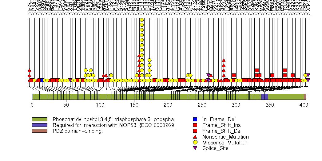
Figure S3. Get High-res Image This figure depicts the distribution of mutations and mutation types across the ARID1A significant gene.
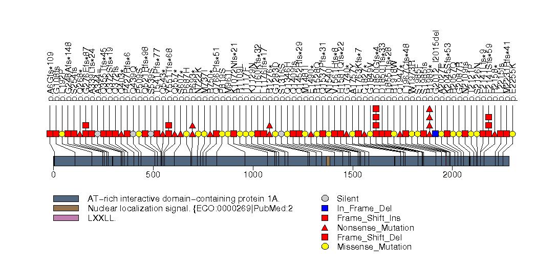
Figure S4. Get High-res Image This figure depicts the distribution of mutations and mutation types across the CTCF significant gene.
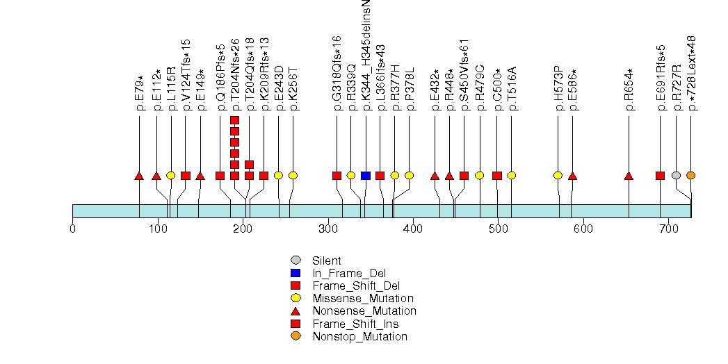
Figure S5. Get High-res Image This figure depicts the distribution of mutations and mutation types across the KRAS significant gene.
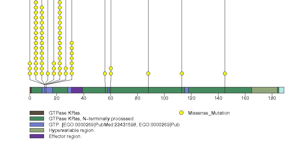
Figure S6. Get High-res Image This figure depicts the distribution of mutations and mutation types across the EGFR significant gene.
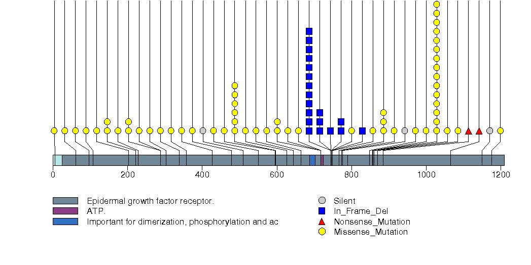
Figure S7. Get High-res Image This figure depicts the distribution of mutations and mutation types across the KMT2D significant gene.

Figure S8. Get High-res Image This figure depicts the distribution of mutations and mutation types across the NF1 significant gene.
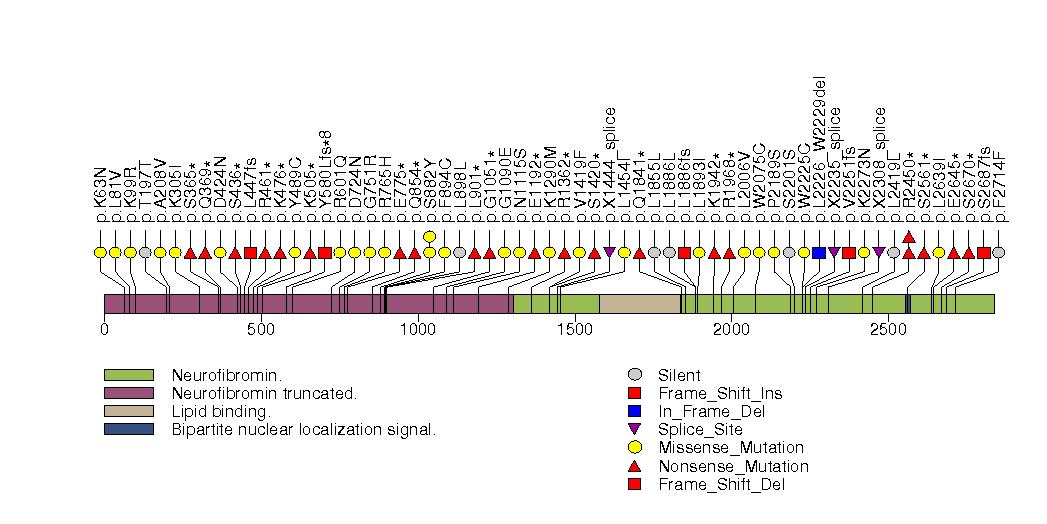
Figure S9. Get High-res Image This figure depicts the distribution of mutations and mutation types across the RPL22 significant gene.

Figure S10. Get High-res Image This figure depicts the distribution of mutations and mutation types across the STK11 significant gene.
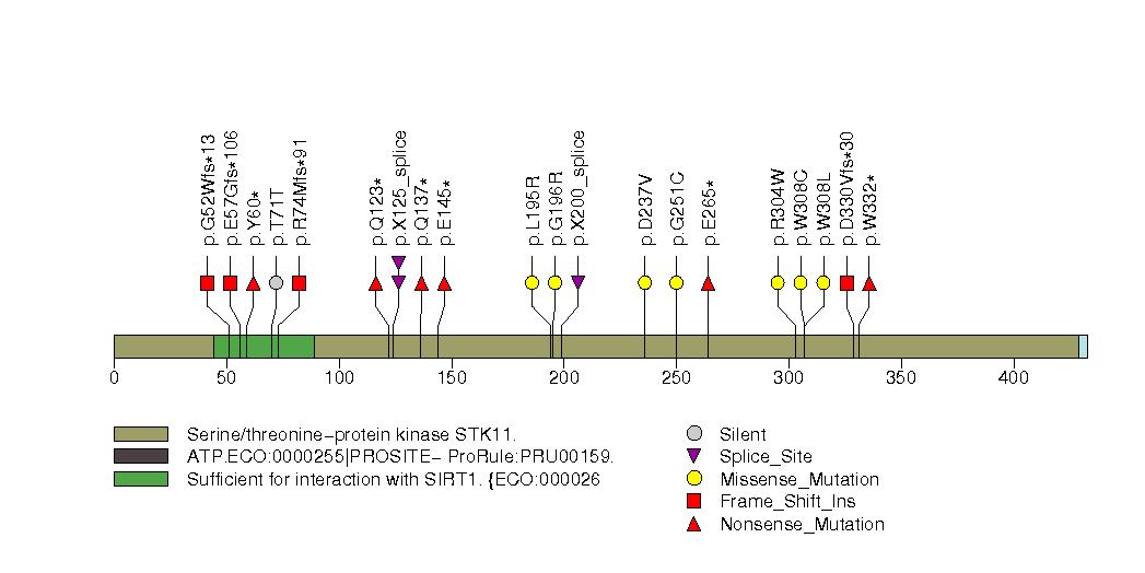
Figure S11. Get High-res Image This figure depicts the distribution of mutations and mutation types across the RB1 significant gene.
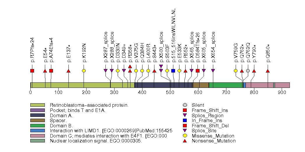
Figure S12. Get High-res Image This figure depicts the distribution of mutations and mutation types across the CDKN2A significant gene.

Figure S13. Get High-res Image This figure depicts the distribution of mutations and mutation types across the PIK3CA significant gene.
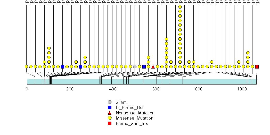
Figure S14. Get High-res Image This figure depicts the distribution of mutations and mutation types across the KEAP1 significant gene.
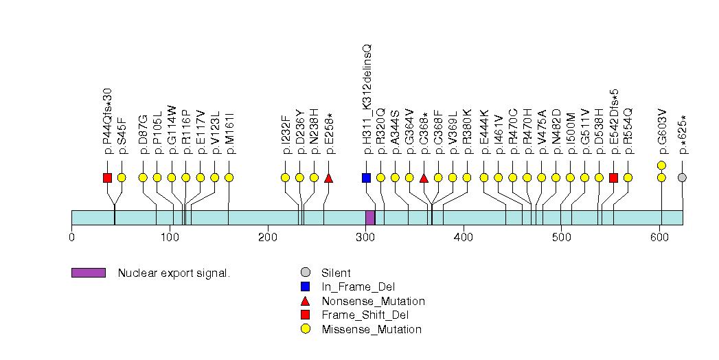
Figure S15. Get High-res Image This figure depicts the distribution of mutations and mutation types across the CTNNB1 significant gene.
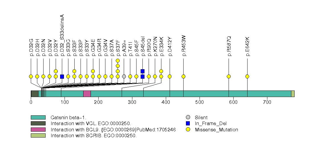
Figure S16. Get High-res Image This figure depicts the distribution of mutations and mutation types across the JAK1 significant gene.
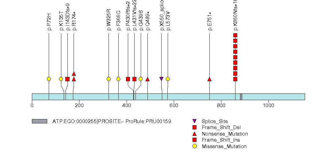
Figure S17. Get High-res Image This figure depicts the distribution of mutations and mutation types across the RNF43 significant gene.
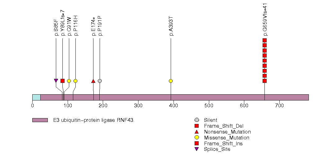
Figure S18. Get High-res Image This figure depicts the distribution of mutations and mutation types across the ZFHX3 significant gene.
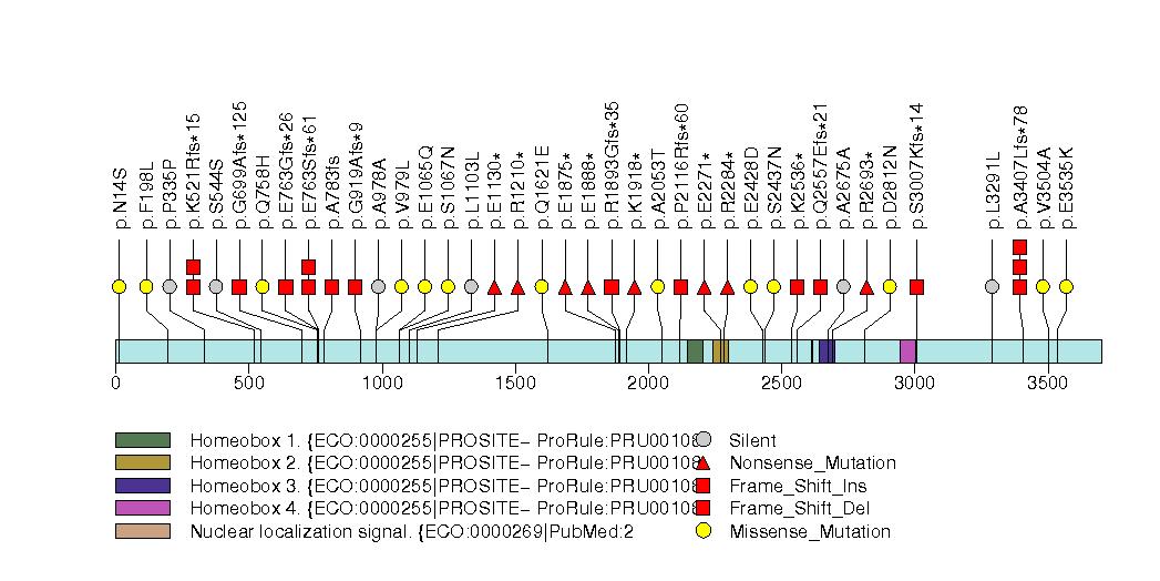
Figure S19. Get High-res Image This figure depicts the distribution of mutations and mutation types across the RPL5 significant gene.
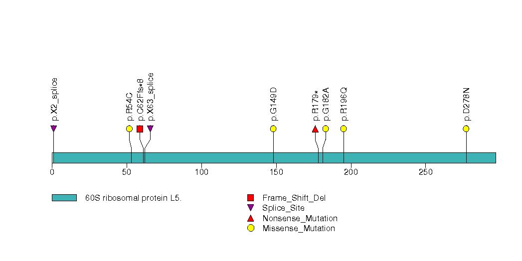
Figure S20. Get High-res Image This figure depicts the distribution of mutations and mutation types across the CUL3 significant gene.
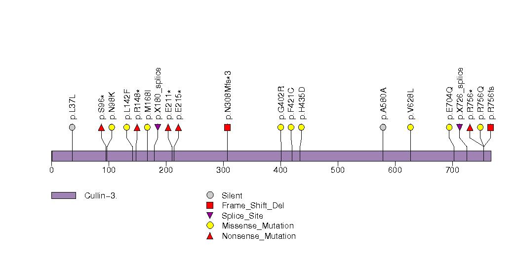
Figure S21. Get High-res Image This figure depicts the distribution of mutations and mutation types across the NSD1 significant gene.
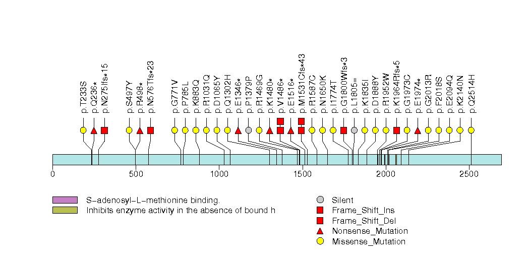
Figure S22. Get High-res Image This figure depicts the distribution of mutations and mutation types across the GLI1 significant gene.
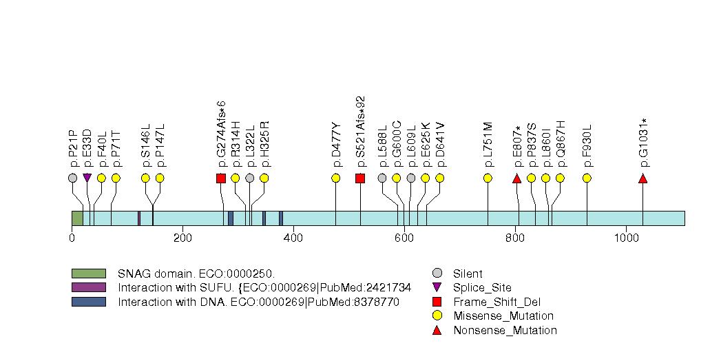
Figure S23. Get High-res Image This figure depicts the distribution of mutations and mutation types across the FBXW7 significant gene.
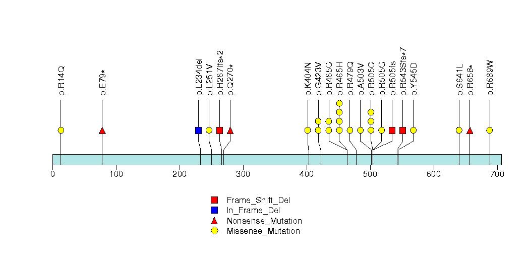
Figure S24. Get High-res Image This figure depicts the distribution of mutations and mutation types across the NOTCH1 significant gene.
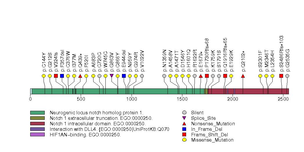
Figure S25. Get High-res Image This figure depicts the distribution of mutations and mutation types across the PPM1D significant gene.
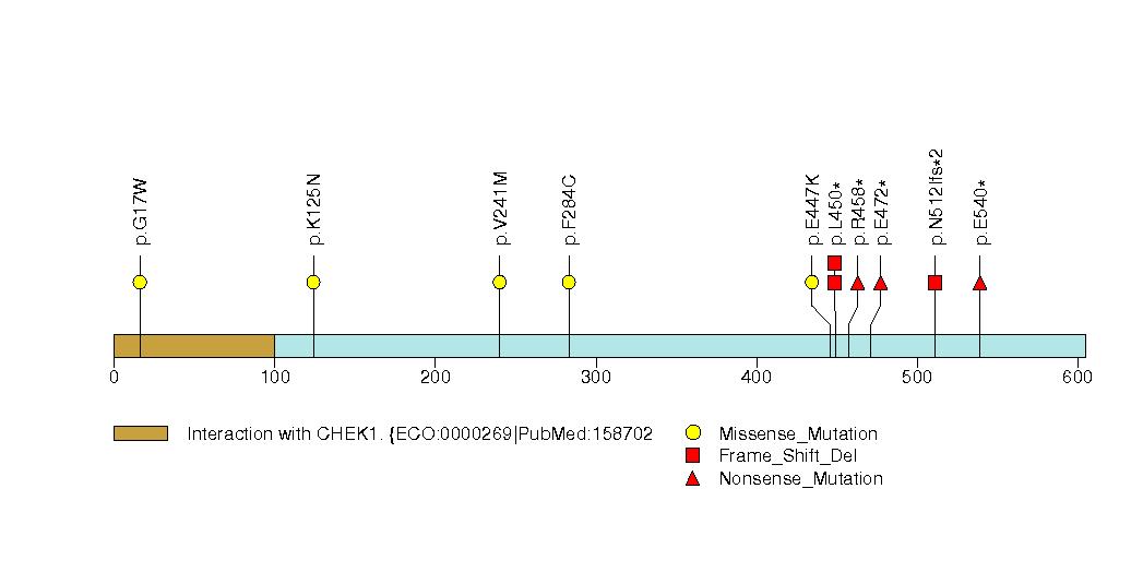
Figure S26. Get High-res Image This figure depicts the distribution of mutations and mutation types across the EIF1AX significant gene.
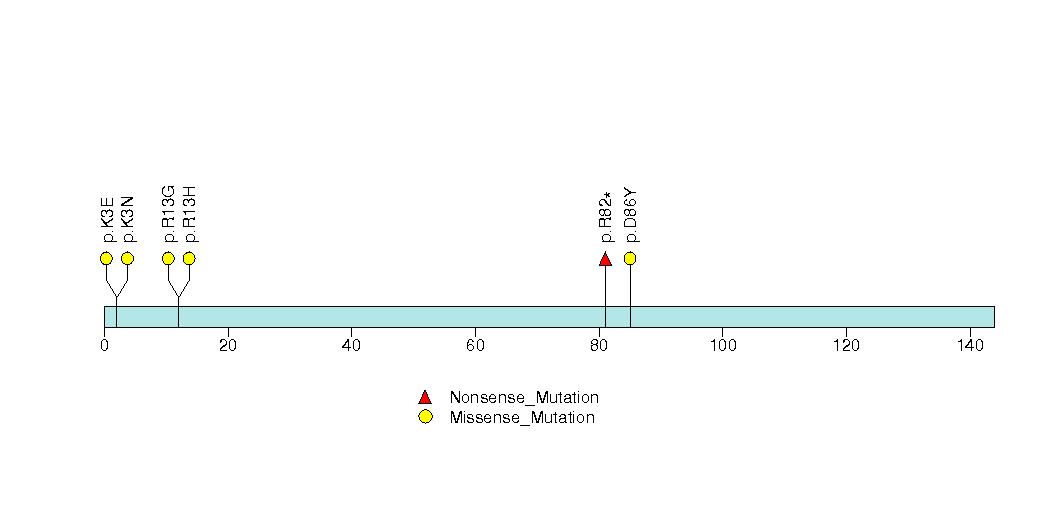
Figure S27. Get High-res Image This figure depicts the distribution of mutations and mutation types across the NFE2L2 significant gene.

Figure S28. Get High-res Image This figure depicts the distribution of mutations and mutation types across the XPO1 significant gene.
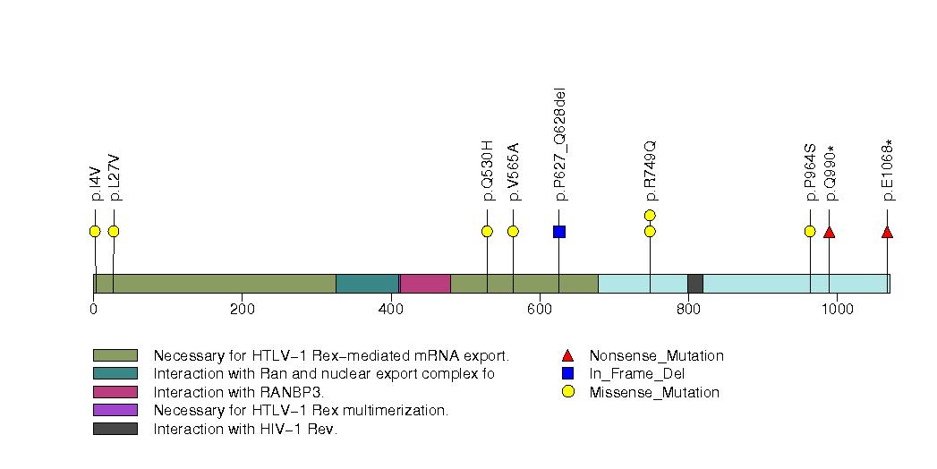
Figure S29. Get High-res Image This figure depicts the distribution of mutations and mutation types across the FGFR4 significant gene.
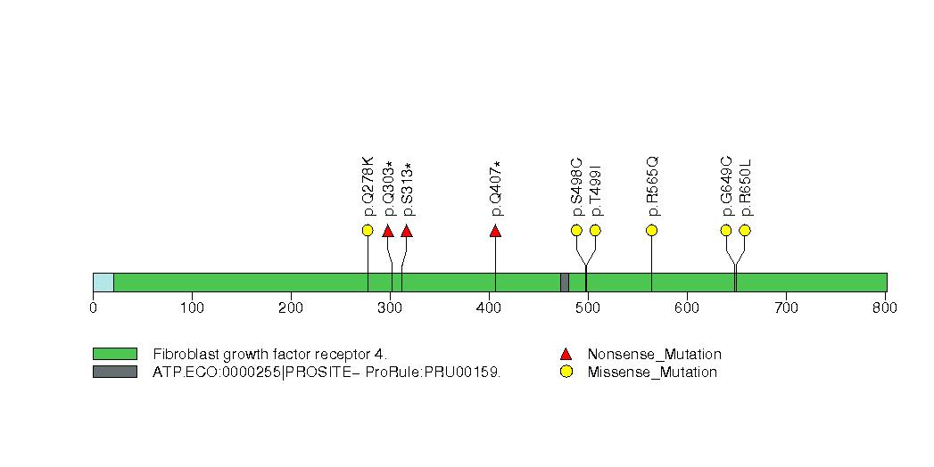
Figure S30. Get High-res Image This figure depicts the distribution of mutations and mutation types across the TFRC significant gene.
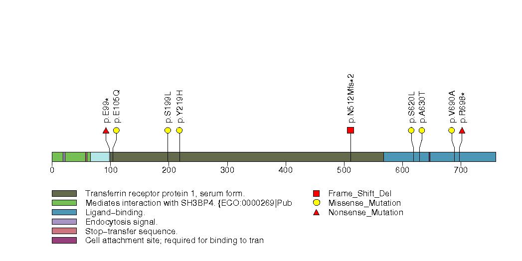
Figure S31. Get High-res Image This figure depicts the distribution of mutations and mutation types across the TCEA1 significant gene.
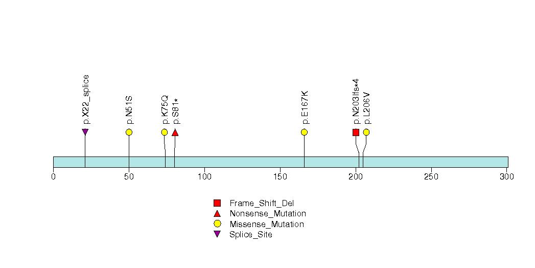
Figure S32. Get High-res Image This figure depicts the distribution of mutations and mutation types across the BCORL1 significant gene.
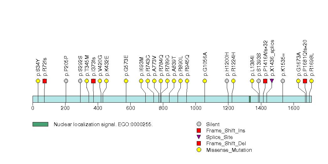
Figure S33. Get High-res Image This figure depicts the distribution of mutations and mutation types across the CHD4 significant gene.
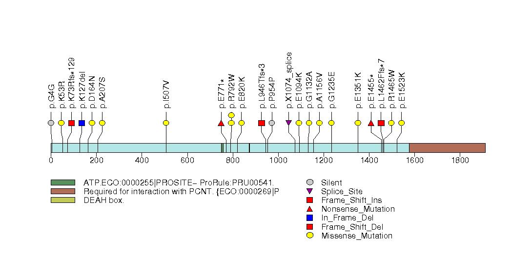
Figure S34. Get High-res Image This figure depicts the distribution of mutations and mutation types across the BTK significant gene.
MutSig and its evolving algorithms have existed since the youth of clinical sequencing, with early versions used in multiple publications. [1][2][3]
"Three significance metrics [are] calculated for each gene, using the […] methods MutSigCV [4], MutSigCL, and MutSigFN [5]. These measure the significance of mutation burden, clustering, and functional impact, respectively […]. MutSigCV determines the P value for observing the given quantity of non-silent mutations in the gene, given the background model determined by silent (and noncoding) mutations in the same gene and the neighbouring genes of covariate space that form its 'bagel'. […] MutSigCL and MutSigFN measure the significance of the positional clustering of the mutations observed, as well as the significance of the tendency for mutations to occur at positions that are highly evolutionarily conserved (using conservation as a proxy for probably functional impact). MutSigCL and MutSigFN are permutation-based methods and their P values are calculated as follows: The observed nonsilent coding mutations in the gene are permuted T times (to simulate the null hypothesis, T = 108 for the most significant genes), randomly reassigning their positions, but preserving their mutational 'category', as determined by local sequence context. We [use] the following context categories: transitions at CpG dinucleotides, transitions at other C-G base pairs, transversions at C-G base pairs, mutations at A-T base pairs, and indels. Indels are unconstrained in terms of where they can move to in the permutations. For each of the random permutations, two scores are calculated: SCL and SFN, measuring the amount of clustering and function impact (measured by conservation) respectively. SCL is defined to be the fraction of mutations occurring in hotspots. A hotspot is defined as a 3-base-pair region of the gene containing many mutations: at least 2, and at least 2% of the total mutations. SFN is defined to be the mean of the base-pair-level conservation values for the position of each non-silent mutation […]. To determine a PCL, the P value for the observed degree of positional clustering, the observed value of SCL (computed for the mutations actually observed), [is] compared to the distribution of SCL obtained from the random permutations, and the P value [is] defined to be the fraction of random permutations in which SCL [is] at least as large as the observed SCL. The P value for the conservation of the mutated positions, PFN, [is] computed analogously." [6]