This pipeline calculates clusters based on a consensus non-negative matrix factorization (NMF) clustering method , . This pipeline has the following features:
-
Convert input data set to a non-negitive matrix by column rank normalization.
-
Classify samples into consensus clusters.
-
Determine differentially expressed marker genes for each subtype.
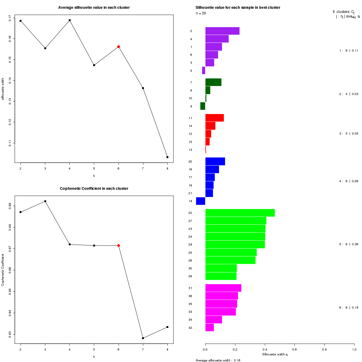
The most robust consensus NMF clustering of 36 samples using the 1500 most variable genes was identified for k = 6 clusters. We computed the clustering for k = 2 to k = 10 and uused the cophenetic correlation coefficient and the average silhouette width calculation to determine the robust clusters.
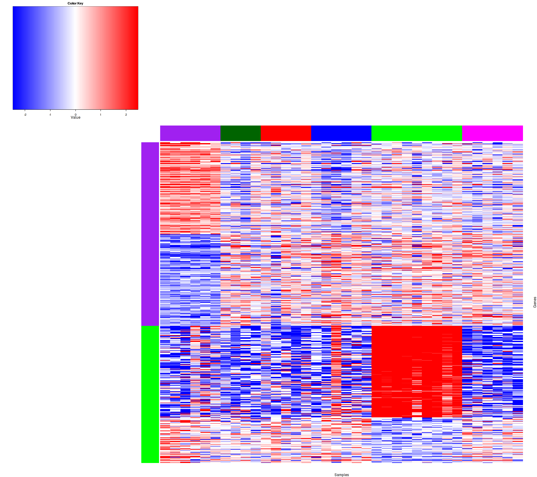
Figure 1. Get High-res Image Samples were separated into 6 clusters. Shown are 36 samples and 524 marker genes. The color bar of the row indicates the marker genes for the corresponding cluster.

Figure 2. Get High-res Image Heatmap with a standard hierarchical clustering for 36 samples and the 1500 most variable genes.

Figure 3. Get High-res Image The silhouette width was calculated for each sample and each value of k. The left upper panel shows the average silhouette width across all samples for each tested k (left upper panel). The left lower panel shows the Cophenetic Correlation Coefficients for each tested k. The right panel shows assignments of clusters to samples and the silhouette width of each sample for the most robust clustering.

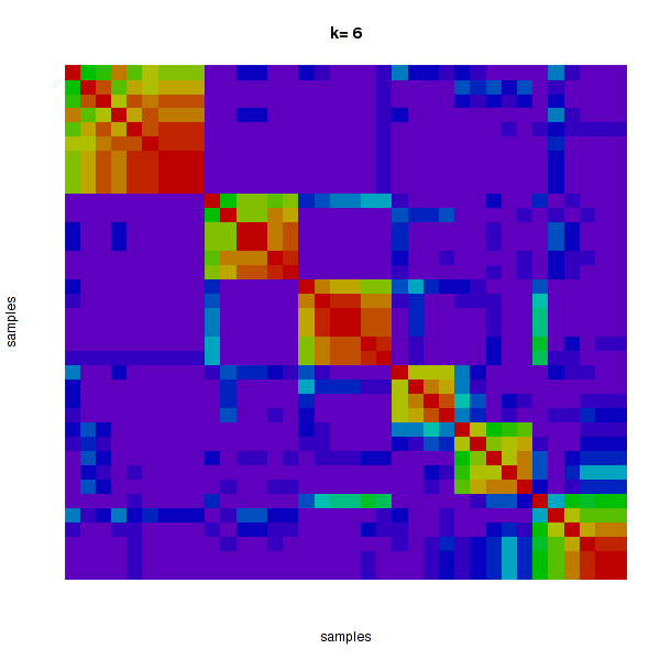
Figure 4. Get High-res Image The consensus matrix after clustering shows 6 clusters with limited overlap between clusters.

Table 1. Get Full Table List of samples with 6 subtypes and silhouette width.
| SampleName | cluster | silhouetteValue |
|---|---|---|
| TCGA-3X-AAV9-01 | 1 | 0.11 |
| TCGA-3X-AAVB-01 | 1 | 0.11 |
| TCGA-3X-AAVC-01 | 1 | 0.23 |
| TCGA-W5-AA2X-01 | 1 | 0.062 |
| TCGA-ZH-A8Y6-01 | 1 | 0.13 |
| TCGA-ZU-A8S4-01 | 1 | 0.093 |
| TCGA-3X-AAVA-01 | 2 | 0.066 |
| TCGA-W5-AA2W-01 | 2 | 0.47 |
| TCGA-W5-AA36-01 | 2 | 0.041 |
| TCGA-W6-AA0S-01 | 2 | -0.063 |
Table 2. Get Full Table List of samples belonging to each cluster in different k clusters.
| SampleName | K=2 | K=3 | K=4 | K=5 | K=6 | K=7 | K=8 |
|---|---|---|---|---|---|---|---|
| TCGA-3X-AAV9-01 | 1 | 1 | 1 | 1 | 1 | 1 | 1 |
| TCGA-3X-AAVA-01 | 1 | 1 | 1 | 2 | 2 | 2 | 2 |
| TCGA-3X-AAVB-01 | 1 | 1 | 1 | 1 | 1 | 1 | 1 |
| TCGA-3X-AAVC-01 | 1 | 1 | 1 | 1 | 1 | 1 | 1 |
| TCGA-3X-AAVE-01 | 1 | 1 | 1 | 1 | 3 | 3 | 3 |
| TCGA-4G-AAZO-01 | 1 | 2 | 2 | 3 | 4 | 4 | 4 |
| TCGA-4G-AAZT-01 | 1 | 2 | 2 | 3 | 4 | 4 | 4 |
| TCGA-W5-AA2H-01 | 1 | 1 | 1 | 1 | 3 | 3 | 6 |
| TCGA-W5-AA2Q-01 | 1 | 2 | 4 | 5 | 6 | 6 | 7 |
| TCGA-W5-AA2R-01 | 1 | 1 | 1 | 2 | 3 | 3 | 3 |
Samples most representative of the clusters, hereby called core samples were identified based on positive silhouette width, indicating higher similarity to their own class than to any other class member. Core samples were used to select differentially expressed marker genes for each subtype by comparing the subclass versus the other subclasses, using Student's t-test.
Table 3. Get Full Table List of marker genes with p <= 0.05 (The positive value of column difference means gene is upregulated in this subtype and vice versa).
| Composite.Element.REF | p | difference | q | subclass |
|---|---|---|---|---|
| ?|10357 | 0.0043 | 0.81 | 0.12 | 1 |
| ?|26823 | 0.0075 | 0.63 | 0.15 | 1 |
| ?|90288 | 0.0073 | -1.6 | 0.15 | 1 |
| AAAS|8086 | 0.0049 | -0.37 | 0.13 | 1 |
| AACSL|729522 | 0.00083 | -2.1 | 0.053 | 1 |
| AACS|65985 | 0.016 | -0.49 | 0.21 | 1 |
| ABCA13|154664 | 0.0091 | 4.3 | 0.16 | 1 |
| ABCA2|20 | 0.012 | -0.83 | 0.19 | 1 |
| ABCC4|10257 | 0.0018 | -1.5 | 0.079 | 1 |
| ABCE1|6059 | 0.024 | 0.53 | 0.25 | 1 |
RSEM is used to estimate gene and transcript abundances and these values are normalized to a fixed upper quaritile value of 1000 for gene and 300 for transcript level estimates. RPKM for a given GeneX is calculated by: (raw read counts * 10^9) / (total reads * length of GeneX). Total reads is the lane yield after removing poor quality reads and the length of GeneX is defined as the median length of all transcripts associated with GeneX.
-
Input file for selecting top 1500 genes = *.uncv2.mRNAseq_RSEM_normalized_log2.txt (quantile normalized RSEM with log2 transformed) / *.mRNAseq_RPKM_log2.txt (RPKM value with log2 transformed) from mRNAseq_preprocess pipeline
-
Input file for the clustering module = /xchip/cga/gdac-prod/tcga-gdac/jobResults/GDAC_TopgenesforCluster/CHOL-TP/22507146/CHOL-TP.expclu.gct
Non-negative matrix factorization (NMF) is an unsupervised learning algorithm that has been shown to identify molecular patterns when applied to gene expression data , . Rather than separating gene clusters based on distance computation, NMF detects contextdependent patterns of gene expression in complex biological systems.
We use the cophenetic correlation coefficients to determine the cluster that yields the most robust clustering. The cophenetic correlation coefficient is computed based on the consensus matrix of the CNMF clustering, and measures how reliably the same samples are assigned to the same cluster across many iterations of the clustering lgorithm with random initializations. The cophenetic correlation coefficients and average silhouette values are used to determine the k with the most robust clusterings. From the plot of cophenetic correlation versus k, we select modes and the the point preceding the greatest decrease in cophenetic correlation coefficient, and from these choose the k with the highest average silhouette value.
Silhouette width is defined as the ratio of average distance of each sample to samples in the same cluster to the smallest distance to samples not in the same cluster. If silhouette width is close to 1, it means that sample is well clustered. If silhouette width is close to -1, it means that sample is misclassified .
In addition to the links below, the full results of the analysis summarized in this report can also be downloaded programmatically using firehose_get, or interactively from either the Broad GDAC website or TCGA Data Coordination Center Portal.