This pipeline calculates clusters based on consensus hierarchical clustering with agglomerative ward linkage[1],[2]. This pipeline has the following features:
-
Classify samples into consensus clusters.
-
Determine differentially expressed marker genes for each subtype.
Median absolute deviation (MAD) was used to select 2500 most variable genes. Consensus ward linkage hierarchical clustering of 100 samples and 2500 genes identified 5 subtypes with the stability of the clustering increasing for k = 2 to k = 10.
Figure 1. Get High-res Image Samples were separated into 5 clusters. Shown are 100 samples and 17868 marker genes. The color bar of the row indicates the marker genes for the corresponding cluster.
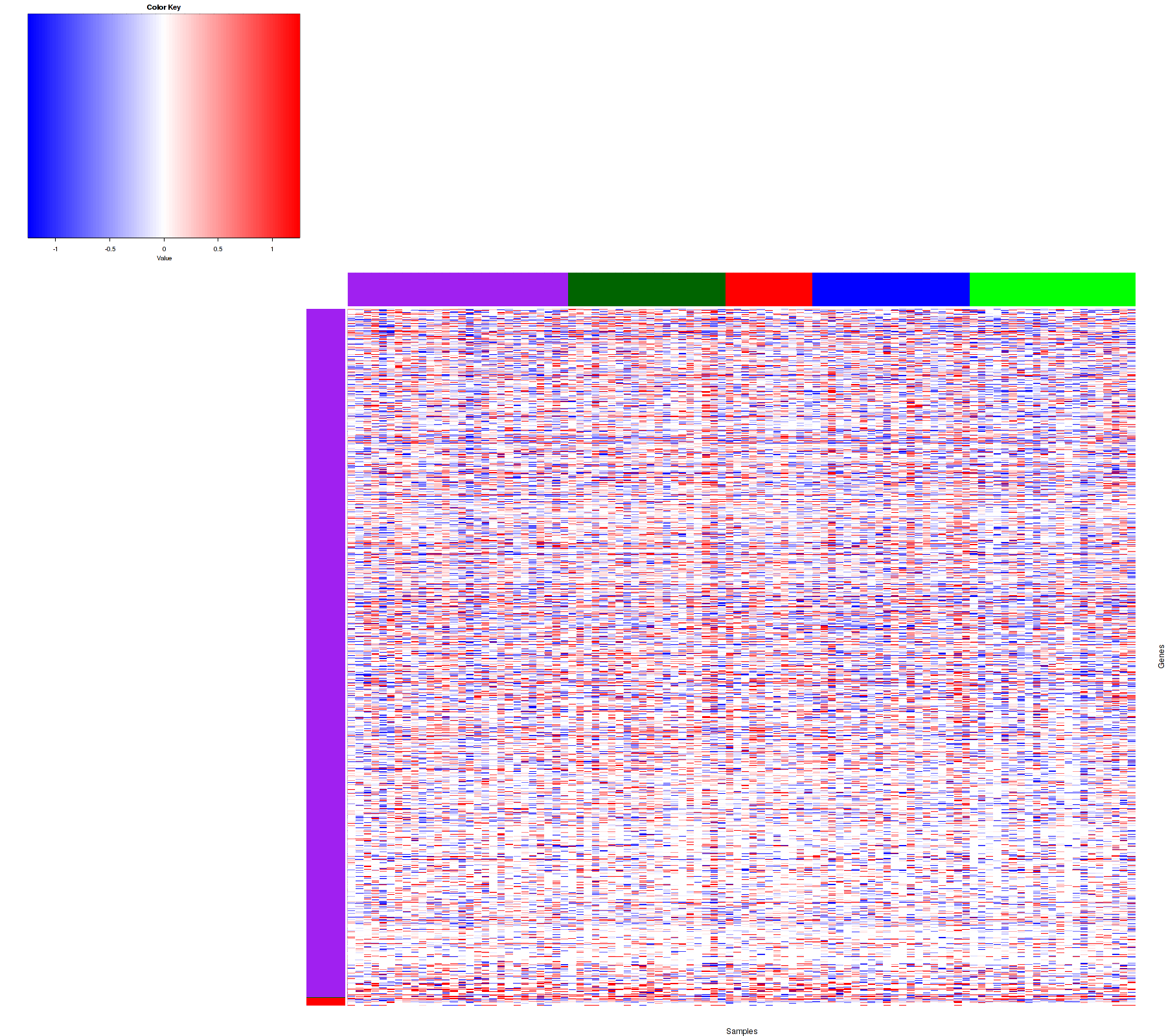
Figure 2. Get High-res Image Heatmap with a standard hierarchical clustering for 100 samples and the 2500 most variable genes. *The NA values were changed to 0 for this figure.
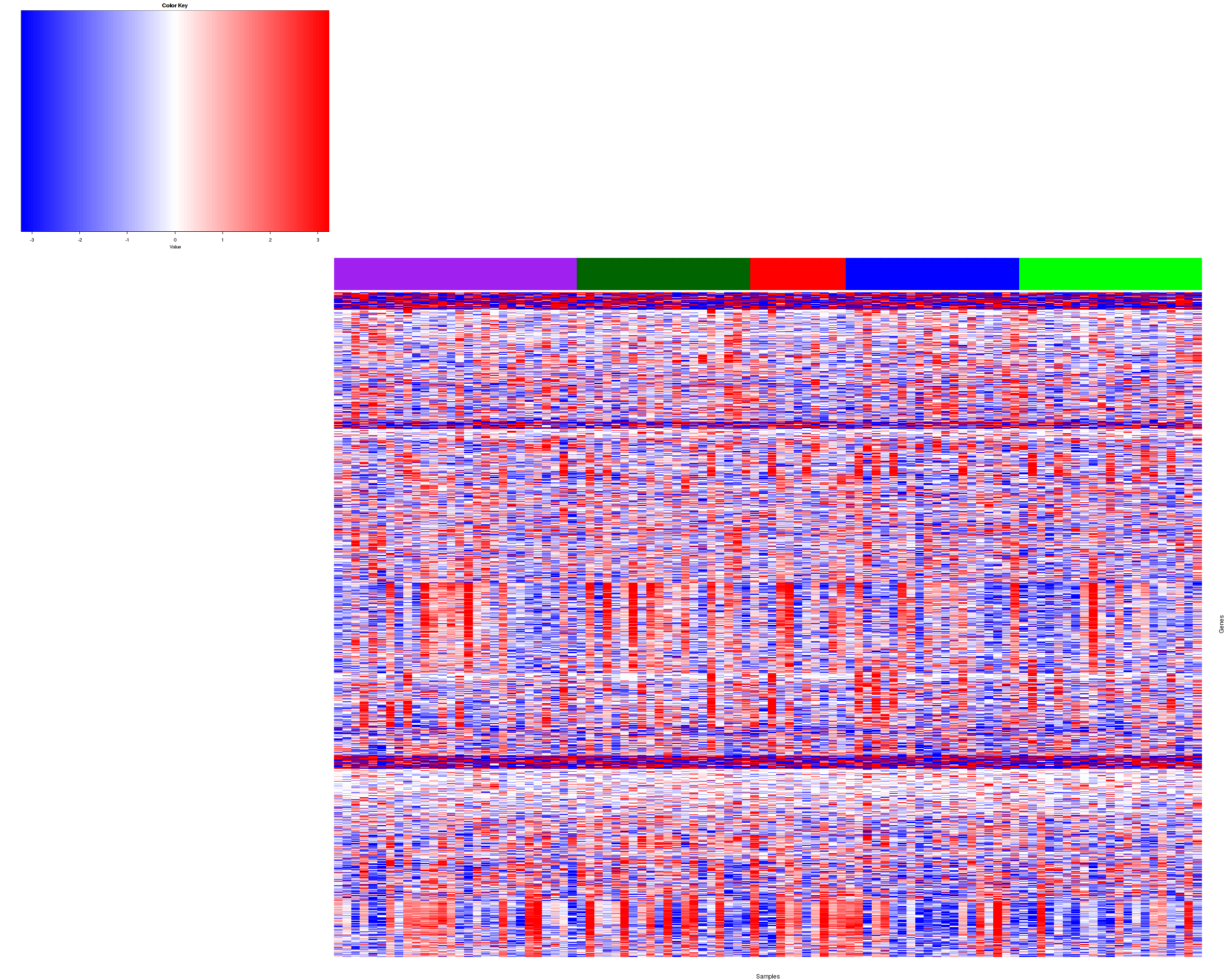
Figure 3. Get High-res Image The silhouette width was calculated for each sample and each value of k. The left upper panel shows the average silhouette width across all samples for each tested k (left upper panel). The left lower panel shows the Cophenetic Correlation Coefficients for each tested k. The right panel shows assignments of clusters to samples and the k silhouette width of each sample for the most robust clustering.
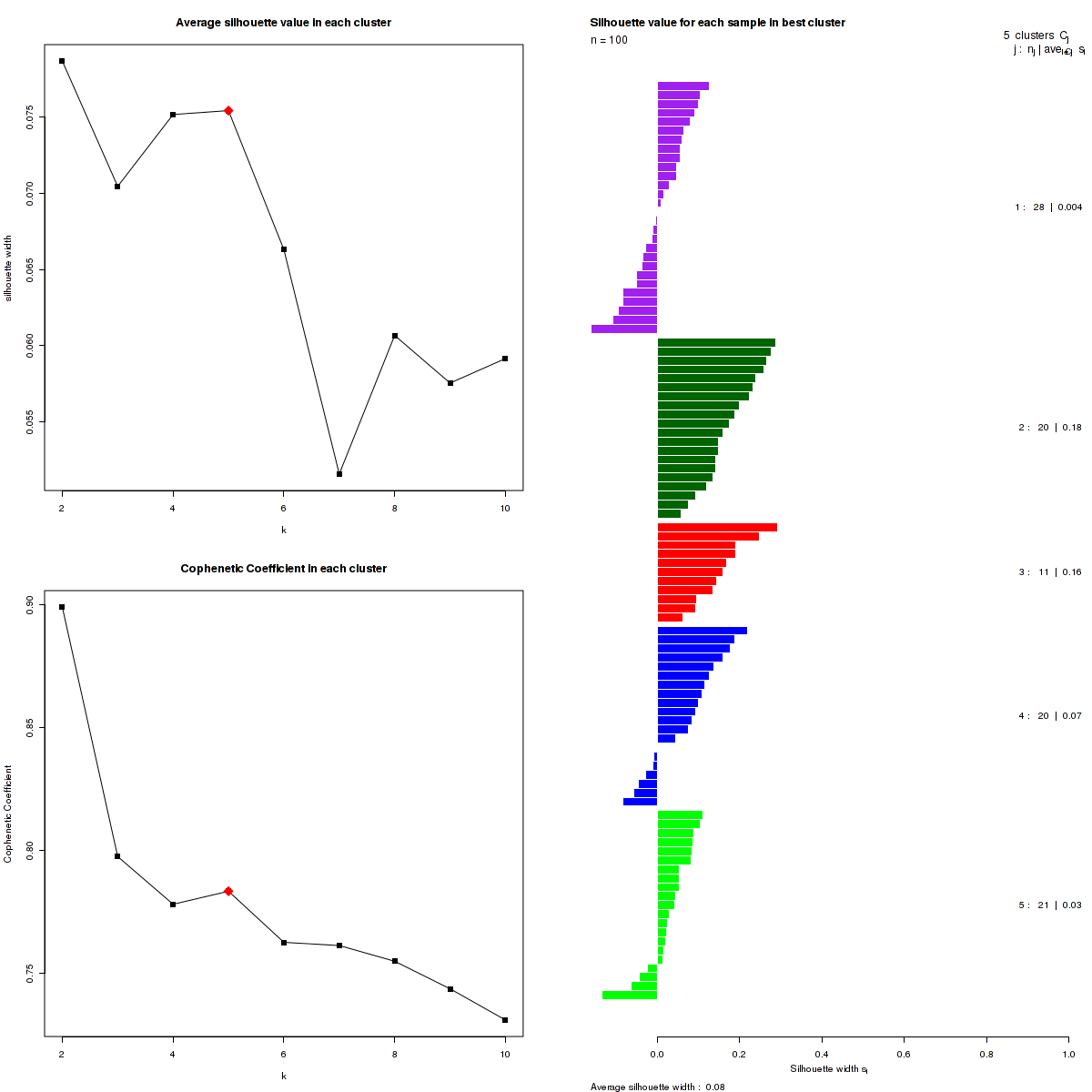
Figure 4. Get High-res Image The consensus matrix after clustering shows 5 clusters with limited overlap between clusters.
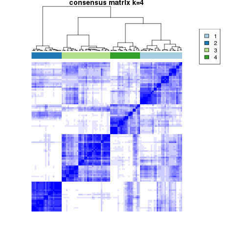
Table 1. Get Full Table List of samples with 5 subtypes and silhouette width.
| SampleName | cluster | silhouetteValue |
|---|---|---|
| C3L-00006_TP | 1 | -0.013 |
| C3L-00137_TP | 1 | 0.22 |
| C3L-00139_TP | 1 | 0.096 |
| C3L-00161_TP | 1 | -0.047 |
| C3L-00356_TP | 1 | 0.017 |
| C3L-00358_TP | 1 | 0.044 |
| C3L-00449_TP | 1 | 0.08 |
| C3L-00601_TP | 1 | 0.092 |
| C3L-00605_TP | 1 | 0.063 |
| C3L-00767_TP | 1 | 0.11 |
Table 2. Get Full Table List of samples belonging to each cluster in different k clusters.
| SampleName | K=2 | K=3 | K=4 | K=5 | K=6 | K=7 | K=8 | K=9 | K=10 |
|---|---|---|---|---|---|---|---|---|---|
| C3L-00006_TP | 1 | 1 | 1 | 1 | 1 | 1 | 1 | 1 | 1 |
| C3L-00008_TP | 2 | 2 | 2 | 2 | 2 | 2 | 2 | 2 | 2 |
| C3L-00032_TP | 1 | 3 | 3 | 3 | 3 | 3 | 3 | 3 | 3 |
| C3L-00090_TP | 1 | 1 | 4 | 4 | 4 | 4 | 4 | 4 | 4 |
| C3L-00098_TP | 1 | 3 | 3 | 5 | 5 | 5 | 5 | 5 | 5 |
| C3L-00136_TP | 1 | 3 | 3 | 5 | 5 | 5 | 5 | 5 | 5 |
| C3L-00137_TP | 1 | 1 | 1 | 1 | 6 | 6 | 6 | 6 | 6 |
| C3L-00139_TP | 1 | 1 | 1 | 1 | 1 | 1 | 1 | 7 | 7 |
| C3L-00143_TP | 1 | 3 | 3 | 3 | 3 | 3 | 3 | 3 | 5 |
| C3L-00145_TP | 1 | 1 | 4 | 4 | 4 | 4 | 7 | 8 | 4 |
Samples most representative of the clusters, hereby called core samples were identified based on positive silhouette width, indicating higher similarity to their own class than to any other class member. Core samples were used to select differentially expressed marker genes for each subtype by comparing the subclass versus the other subclasses, using Student's t-test.
Table 3. Get Full Table List of marker genes with p <= 0.05 (The positive value of column difference means gene is upregulated in this subtype and vice versa).
| Hybridization.REF | p | difference | q | subclass |
|---|---|---|---|---|
| TSPAN6|ENSG00000000003.13 | 0.56 | 0.074 | 1 | 1 |
| TNMD|ENSG00000000005.5 | 0.12 | 0.84 | 1 | 1 |
| DPM1|ENSG00000000419.11 | 0.64 | 0.064 | 1 | 1 |
| SCYL3|ENSG00000000457.12 | 0.58 | -0.081 | 1 | 1 |
| C1ORF112|ENSG00000000460.15 | 0.45 | 0.13 | 1 | 1 |
| FGR|ENSG00000000938.11 | 0.95 | -0.018 | 1 | 1 |
| CFH|ENSG00000000971.14 | 0.27 | -0.35 | 1 | 1 |
| FUCA2|ENSG00000001036.12 | 0.52 | -0.093 | 1 | 1 |
| GCLC|ENSG00000001084.9 | 0.72 | -0.077 | 1 | 1 |
| NFYA|ENSG00000001167.13 | 0.45 | 0.086 | 1 | 1 |
FPKM-UQ with log2 transformed is as the input data for the clustering. FPKM-UQ = (C x 109)/(UQ x L) where UQ= upper quartile of fragment count to autosomal protein coding, L = Length of Gene (aggregate exons), C = Fragment Count
-
Input file = CPTAC3-UCEC-TP.expclu.gct
Consensus Hierarchical clustering is a resampling-based clustering. It provides for a method to represent the consensus across multiple runs of a clustering algorithm and to assess the stability of the discovered clusters. To this end, perturbations of the original data are simulated by resampling techniques [1],[2].
Silhouette width is defined as the ratio of average distance of each sample to samples in the same cluster to the smallest distance to samples not in the same cluster. If silhouette width is close to 1, it means that sample is well clustered. If silhouette width is close to -1, it means that sample is misclassified[3][5].
The cophenetic correlation coefficient is computed as the Pearson correlation of two distance matrices:
-
Distance between samples induced by the consensus matrix.
-
Distance between samples induced by the linkage used in reordering the consensus matrix.
The cophenetic correlation coefficients and average silhouette values are used to determine the k with the most robust clusterings. From the plot of cophenetic correlation versus k, we select modes and the the point preceding the greatest decrease in cophenetic correlation coefficient, and from these choose the k with the highest average silhouette value.