Correlation between aggregated molecular cancer subtypes and selected clinical features

Lung Adenocarcinoma (Primary solid tumor)

17 April 2019 | None

Maintainer Information

Maintained by Broad Institute GDAC (Broad Institute of MIT & Harvard)

Overview

Introduction

This pipeline computes the correlation between cancer subtypes identified by different molecular patterns and selected clinical features.

Summary

Testing the association between subtypes identified by 2 different clustering approaches and 17 clinical features across 111 patients, 11 significant findings detected with P value < 0.05 and Q value < 0.25.

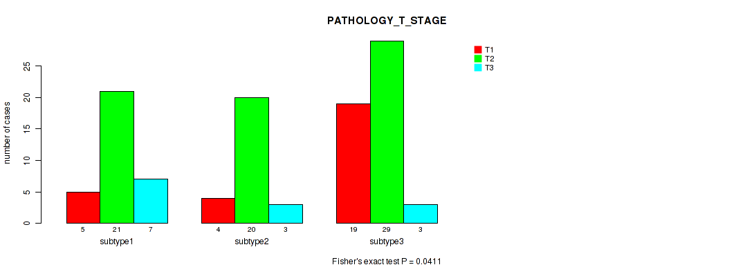
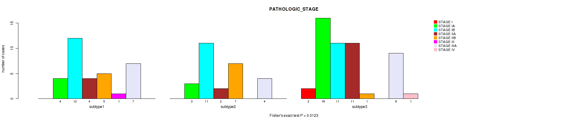
Consensus hierarchical clustering analysis on array-based mRNA expression data identified 3 subtypes that correlate to 'HISTOLOGIC_GRADE', 'PATHOLOGY_T_STAGE', 'PATHOLOGIC_STAGE', 'GENDER', 'COUNTRY_OF_ORIGIN', and 'ORIGIN_ASIA'.
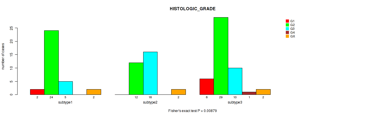
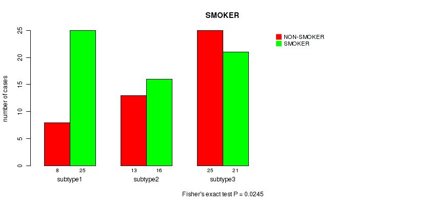
3 subtypes identified in current cancer cohort by 'LINCRNA CHIERARCHICAL'. These subtypes correlate to 'HISTOLOGIC_GRADE', 'GENDER', 'SMOKER', 'COUNTRY_OF_ORIGIN', and 'ORIGIN_ASIA'.

Results

Overview of the results

Table 1. Get Full Table Overview of the association between subtypes identified by 2 different clustering approaches and 17 clinical features. Shown in the table are P values (Q values). Thresholded by P value < 0.05 and Q value < 0.25, 11 significant findings detected.


Clinical Features	Statistical Tests	mRNA cHierClus subtypes	LINCRNA CHIERARCHICAL
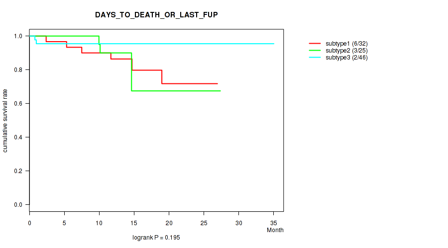
DAYS TO DEATH OR LAST FUP	logrank test	0.195 (0.331)	0.239 (0.387)
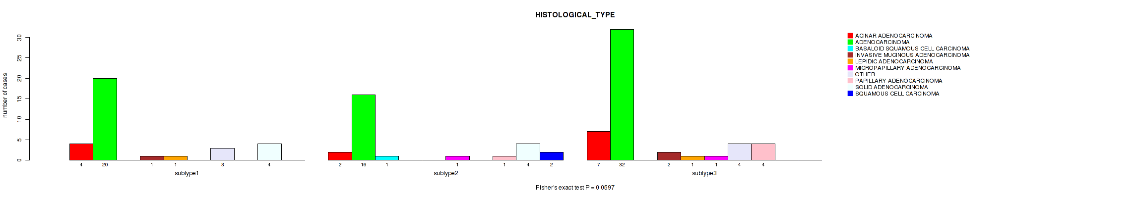
HISTOLOGICAL TYPE	Fisher's exact test	0.0597 (0.156)	0.295 (0.436)
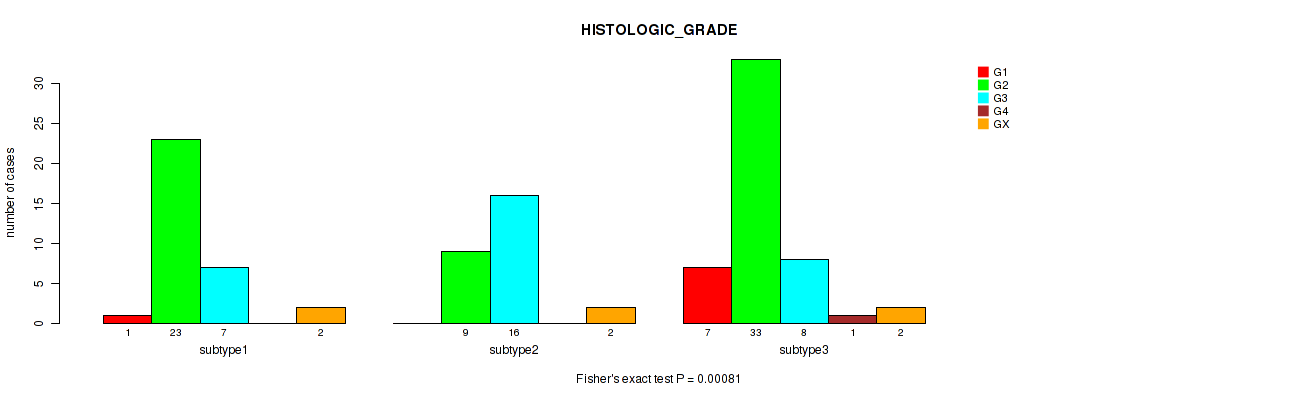
HISTOLOGIC GRADE	Fisher's exact test	0.00081 (0.00688)	0.00879 (0.046)
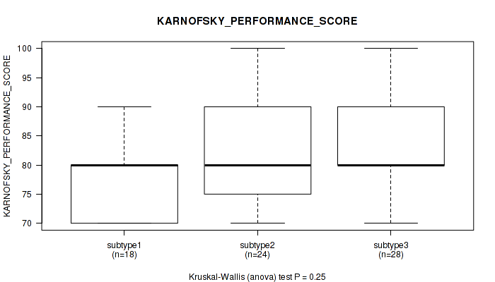
KARNOFSKY PERFORMANCE SCORE	Kruskal-Wallis (anova)	0.25 (0.387)	0.105 (0.239)
PATHOLOGY T STAGE	Fisher's exact test	0.0411 (0.127)	0.136 (0.273)
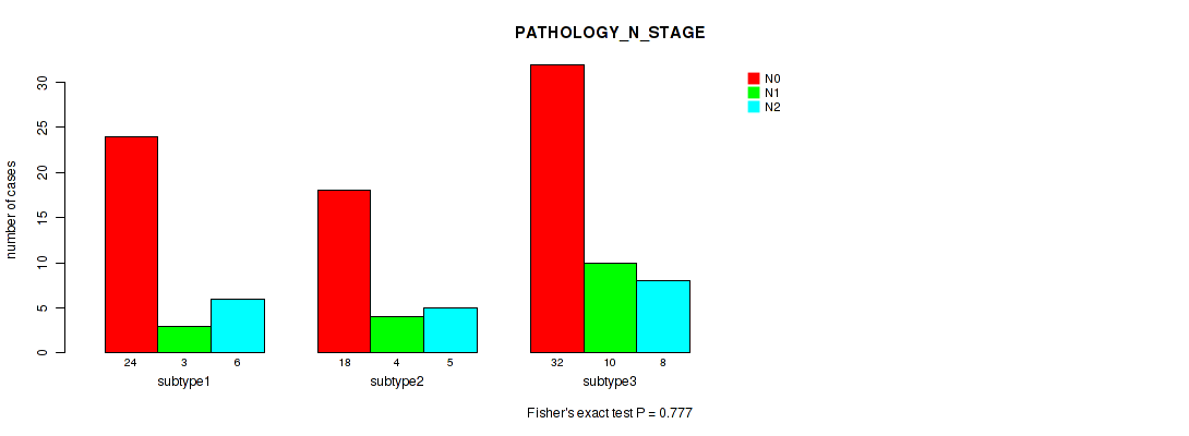
PATHOLOGY N STAGE	Fisher's exact test	0.777 (0.915)	0.78 (0.915)
PATHOLOGIC STAGE	Fisher's exact test	0.0123 (0.0521)	0.0656 (0.159)
YEARS TO BIRTH	Kruskal-Wallis (anova)	0.627 (0.79)	0.177 (0.317)
ETHNICITY	Fisher's exact test	1 (1.00)	1 (1.00)
GENDER	Fisher's exact test	2e-05 (0.00034)	1e-05 (0.00034)
RACE	Fisher's exact test	0.852 (0.966)	0.58 (0.758)
RADIATION THERAPY	Fisher's exact test	0.55 (0.747)	0.371 (0.525)
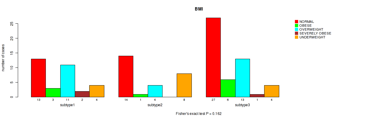
BMI	Fisher's exact test	0.162 (0.307)	0.134 (0.273)
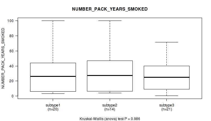
NUMBER PACK YEARS SMOKED	Kruskal-Wallis (anova)	0.986 (1.00)	0.945 (1.00)
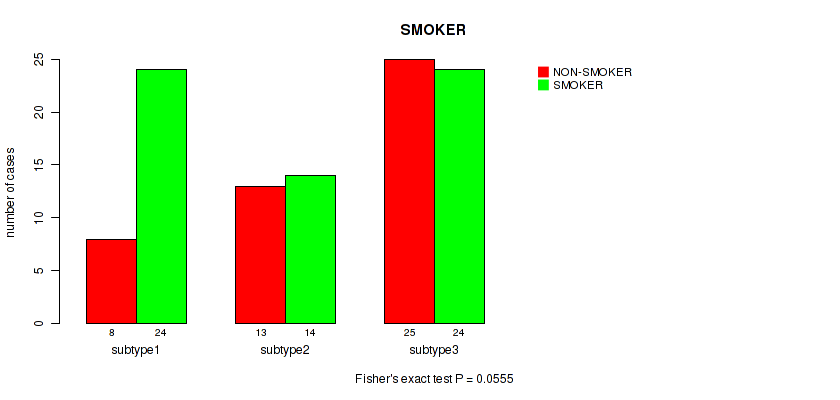
SMOKER	Fisher's exact test	0.0555 (0.156)	0.0245 (0.0926)
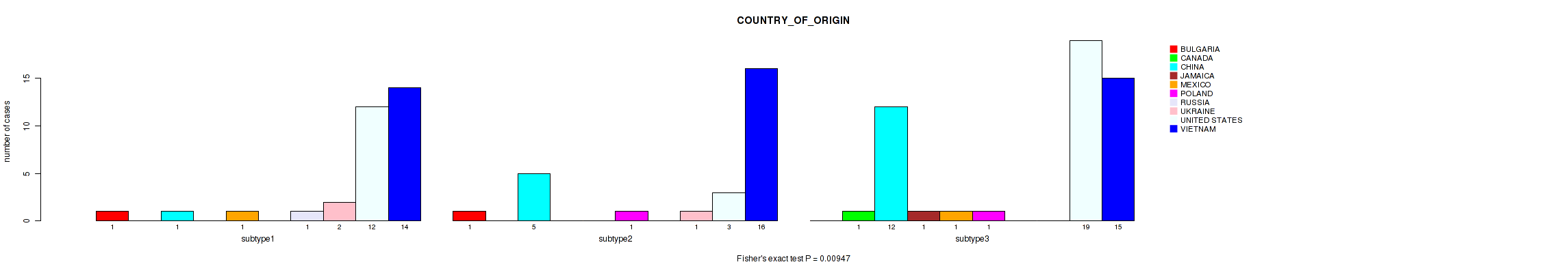
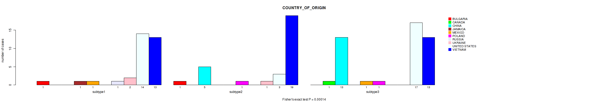
COUNTRY OF ORIGIN	Fisher's exact test	0.00947 (0.046)	0.00014 (0.00159)
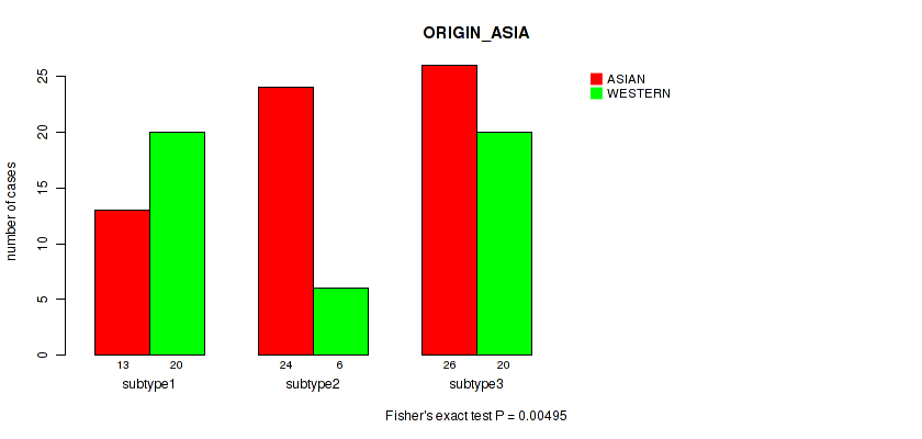
ORIGIN ASIA	Fisher's exact test	0.0388 (0.127)	0.00495 (0.0337)

Clustering Approach #1: 'mRNA cHierClus subtypes'

Table S1. Description of clustering approach #1: 'mRNA cHierClus subtypes'

Cluster Labels	1	2	3
Number of samples	33	27	51

'mRNA cHierClus subtypes' versus 'DAYS_TO_DEATH_OR_LAST_FUP'

P value = 0.195 (logrank test), Q value = 0.33

Table S2. Clustering Approach #1: 'mRNA cHierClus subtypes' versus Clinical Feature #1: 'DAYS_TO_DEATH_OR_LAST_FUP'

	nPatients	nDeath	Duration Range (Median), Month
ALL	111	11	0.2 - 35.0 (13.1)
subtype1	32	6	1.4 - 26.9 (13.9)
subtype2	25	3	0.2 - 27.4 (12.9)
subtype3	46	2	0.5 - 35.0 (12.2)

Figure S1. Get High-res Image Clustering Approach #1: 'mRNA cHierClus subtypes' versus Clinical Feature #1: 'DAYS_TO_DEATH_OR_LAST_FUP'

'mRNA cHierClus subtypes' versus 'HISTOLOGICAL_TYPE'

P value = 0.0597 (Fisher's exact test), Q value = 0.16

Table S3. Clustering Approach #1: 'mRNA cHierClus subtypes' versus Clinical Feature #2: 'HISTOLOGICAL_TYPE'

nPatients	ACINAR ADENOCARCINOMA	ADENOCARCINOMA	BASALOID SQUAMOUS CELL CARCINOMA	INVASIVE MUCINOUS ADENOCARCINOMA	LEPIDIC ADENOCARCINOMA	MICROPAPILLARY ADENOCARCINOMA	OTHER	PAPILLARY ADENOCARCINOMA	SOLID ADENOCARCINOMA	SQUAMOUS CELL CARCINOMA
ALL	13	68	1	3	2	2	7	5	8	2
subtype1	4	20	0	1	1	0	3	0	4	0
subtype2	2	16	1	0	0	1	0	1	4	2
subtype3	7	32	0	2	1	1	4	4	0	0

Figure S2. Get High-res Image Clustering Approach #1: 'mRNA cHierClus subtypes' versus Clinical Feature #2: 'HISTOLOGICAL_TYPE'

'mRNA cHierClus subtypes' versus 'HISTOLOGIC_GRADE'

P value = 0.00081 (Fisher's exact test), Q value = 0.0069

Table S4. Clustering Approach #1: 'mRNA cHierClus subtypes' versus Clinical Feature #3: 'HISTOLOGIC_GRADE'

nPatients	G1	G2	G3	G4	GX
ALL	8	65	31	1	6
subtype1	1	23	7	0	2
subtype2	0	9	16	0	2
subtype3	7	33	8	1	2

Figure S3. Get High-res Image Clustering Approach #1: 'mRNA cHierClus subtypes' versus Clinical Feature #3: 'HISTOLOGIC_GRADE'

'mRNA cHierClus subtypes' versus 'KARNOFSKY_PERFORMANCE_SCORE'

P value = 0.25 (Kruskal-Wallis (anova)), Q value = 0.39

Table S5. Clustering Approach #1: 'mRNA cHierClus subtypes' versus Clinical Feature #4: 'KARNOFSKY_PERFORMANCE_SCORE'

	nPatients	Mean (Std.Dev)
ALL	70	81.7 (9.0)
subtype1	18	78.9 (7.6)
subtype2	24	81.7 (9.2)
subtype3	28	83.6 (9.5)

Figure S4. Get High-res Image Clustering Approach #1: 'mRNA cHierClus subtypes' versus Clinical Feature #4: 'KARNOFSKY_PERFORMANCE_SCORE'

'mRNA cHierClus subtypes' versus 'PATHOLOGY_T_STAGE'

P value = 0.0411 (Kruskal-Wallis (anova)), Q value = 0.13

Table S6. Clustering Approach #1: 'mRNA cHierClus subtypes' versus Clinical Feature #5: 'PATHOLOGY_T_STAGE'

	T1	T2	T3
ALL	28	70	13
subtype1	5	21	7
subtype2	4	20	3
subtype3	19	29	3

Figure S5. Get High-res Image Clustering Approach #1: 'mRNA cHierClus subtypes' versus Clinical Feature #5: 'PATHOLOGY_T_STAGE'

'mRNA cHierClus subtypes' versus 'PATHOLOGY_N_STAGE'

P value = 0.777 (Kruskal-Wallis (anova)), Q value = 0.91

Table S7. Clustering Approach #1: 'mRNA cHierClus subtypes' versus Clinical Feature #6: 'PATHOLOGY_N_STAGE'

	N0	N1	N2
ALL	74	17	19
subtype1	24	3	6
subtype2	18	4	5
subtype3	32	10	8

Figure S6. Get High-res Image Clustering Approach #1: 'mRNA cHierClus subtypes' versus Clinical Feature #6: 'PATHOLOGY_N_STAGE'

'mRNA cHierClus subtypes' versus 'PATHOLOGIC_STAGE'

P value = 0.0123 (Fisher's exact test), Q value = 0.052

Table S8. Clustering Approach #1: 'mRNA cHierClus subtypes' versus Clinical Feature #7: 'PATHOLOGIC_STAGE'

nPatients	STAGE I	STAGE IA	STAGE IB	STAGE IIA	STAGE IIB	STAGE III	STAGE IIIA	STAGE IV
ALL	2	23	34	17	13	1	20	1
subtype1	0	4	12	4	5	1	7	0
subtype2	0	3	11	2	7	0	4	0
subtype3	2	16	11	11	1	0	9	1

Figure S7. Get High-res Image Clustering Approach #1: 'mRNA cHierClus subtypes' versus Clinical Feature #7: 'PATHOLOGIC_STAGE'

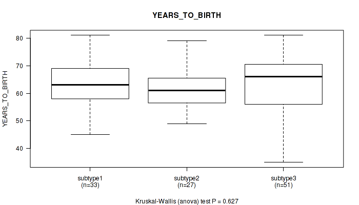
'mRNA cHierClus subtypes' versus 'YEARS_TO_BIRTH'

P value = 0.627 (Kruskal-Wallis (anova)), Q value = 0.79

Table S9. Clustering Approach #1: 'mRNA cHierClus subtypes' versus Clinical Feature #8: 'YEARS_TO_BIRTH'

	nPatients	Mean (Std.Dev)
ALL	111	62.6 (9.6)
subtype1	33	63.4 (8.4)
subtype2	27	61.8 (7.5)
subtype3	51	62.5 (11.3)

Figure S8. Get High-res Image Clustering Approach #1: 'mRNA cHierClus subtypes' versus Clinical Feature #8: 'YEARS_TO_BIRTH'

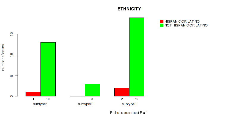
'mRNA cHierClus subtypes' versus 'ETHNICITY'

P value = 1 (Fisher's exact test), Q value = 1

Table S10. Clustering Approach #1: 'mRNA cHierClus subtypes' versus Clinical Feature #9: 'ETHNICITY'

nPatients	HISPANIC OR LATINO	NOT HISPANIC OR LATINO
ALL	3	35
subtype1	1	13
subtype2	0	3
subtype3	2	19

Figure S9. Get High-res Image Clustering Approach #1: 'mRNA cHierClus subtypes' versus Clinical Feature #9: 'ETHNICITY'

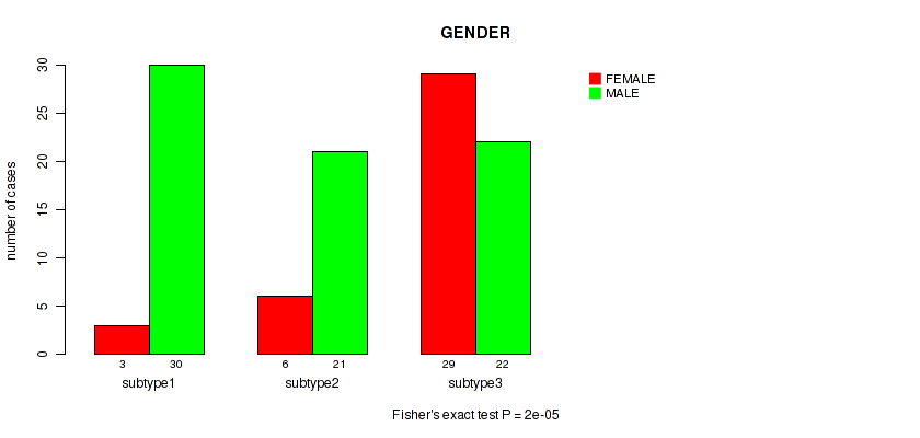
'mRNA cHierClus subtypes' versus 'GENDER'

P value = 2e-05 (Fisher's exact test), Q value = 0.00034

Table S11. Clustering Approach #1: 'mRNA cHierClus subtypes' versus Clinical Feature #10: 'GENDER'

nPatients	FEMALE	MALE
ALL	38	73
subtype1	3	30
subtype2	6	21
subtype3	29	22

Figure S10. Get High-res Image Clustering Approach #1: 'mRNA cHierClus subtypes' versus Clinical Feature #10: 'GENDER'

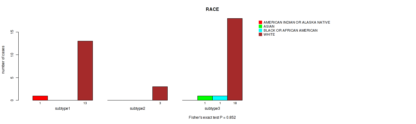
'mRNA cHierClus subtypes' versus 'RACE'

P value = 0.852 (Fisher's exact test), Q value = 0.97

Table S12. Clustering Approach #1: 'mRNA cHierClus subtypes' versus Clinical Feature #11: 'RACE'

nPatients	AMERICAN INDIAN OR ALASKA NATIVE	ASIAN	BLACK OR AFRICAN AMERICAN	WHITE
ALL	1	1	1	34
subtype1	1	0	0	13
subtype2	0	0	0	3
subtype3	0	1	1	18

Figure S11. Get High-res Image Clustering Approach #1: 'mRNA cHierClus subtypes' versus Clinical Feature #11: 'RACE'

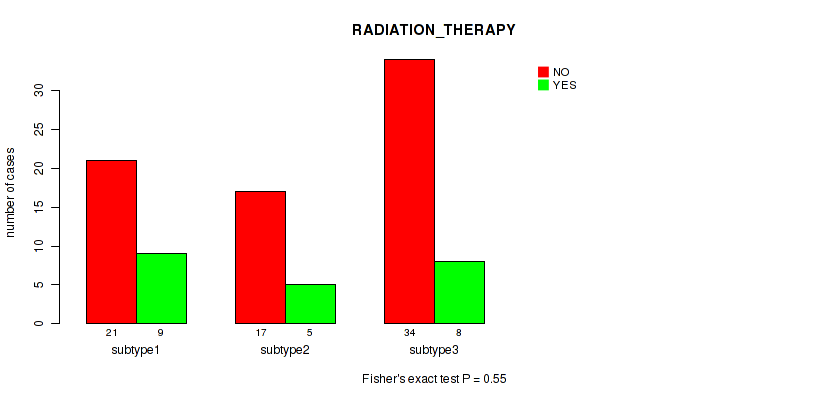
'mRNA cHierClus subtypes' versus 'RADIATION_THERAPY'

P value = 0.55 (Fisher's exact test), Q value = 0.75

Table S13. Clustering Approach #1: 'mRNA cHierClus subtypes' versus Clinical Feature #12: 'RADIATION_THERAPY'

nPatients	NO	YES
ALL	72	22
subtype1	21	9
subtype2	17	5
subtype3	34	8

Figure S12. Get High-res Image Clustering Approach #1: 'mRNA cHierClus subtypes' versus Clinical Feature #12: 'RADIATION_THERAPY'

'mRNA cHierClus subtypes' versus 'BMI'

P value = 0.162 (Fisher's exact test), Q value = 0.31

Table S14. Clustering Approach #1: 'mRNA cHierClus subtypes' versus Clinical Feature #13: 'BMI'

nPatients	NORMAL	OBESE	OVERWEIGHT	SEVERELY OBESE	UNDERWEIGHT
ALL	54	10	28	3	16
subtype1	13	3	11	2	4
subtype2	14	1	4	0	8
subtype3	27	6	13	1	4

Figure S13. Get High-res Image Clustering Approach #1: 'mRNA cHierClus subtypes' versus Clinical Feature #13: 'BMI'

'mRNA cHierClus subtypes' versus 'NUMBER_PACK_YEARS_SMOKED'

P value = 0.986 (Kruskal-Wallis (anova)), Q value = 1

Table S15. Clustering Approach #1: 'mRNA cHierClus subtypes' versus Clinical Feature #14: 'NUMBER_PACK_YEARS_SMOKED'

	nPatients	Mean (Std.Dev)
ALL	55	27.4 (23.4)
subtype1	20	28.2 (25.1)
subtype2	14	28.9 (27.5)
subtype3	21	25.7 (19.6)

Figure S14. Get High-res Image Clustering Approach #1: 'mRNA cHierClus subtypes' versus Clinical Feature #14: 'NUMBER_PACK_YEARS_SMOKED'

'mRNA cHierClus subtypes' versus 'SMOKER'

P value = 0.0555 (Fisher's exact test), Q value = 0.16

Table S16. Clustering Approach #1: 'mRNA cHierClus subtypes' versus Clinical Feature #15: 'SMOKER'

nPatients	NON-SMOKER	SMOKER
ALL	46	62
subtype1	8	24
subtype2	13	14
subtype3	25	24

Figure S15. Get High-res Image Clustering Approach #1: 'mRNA cHierClus subtypes' versus Clinical Feature #15: 'SMOKER'

'mRNA cHierClus subtypes' versus 'COUNTRY_OF_ORIGIN'

P value = 0.00947 (Fisher's exact test), Q value = 0.046

Table S17. Clustering Approach #1: 'mRNA cHierClus subtypes' versus Clinical Feature #16: 'COUNTRY_OF_ORIGIN'

nPatients	BULGARIA	CANADA	CHINA	JAMAICA	MEXICO	POLAND	RUSSIA	UKRAINE	UNITED STATES	VIETNAM
ALL	2	1	18	1	2	2	1	3	34	45
subtype1	1	0	1	0	1	0	1	2	12	14
subtype2	1	0	5	0	0	1	0	1	3	16
subtype3	0	1	12	1	1	1	0	0	19	15

Figure S16. Get High-res Image Clustering Approach #1: 'mRNA cHierClus subtypes' versus Clinical Feature #16: 'COUNTRY_OF_ORIGIN'

'mRNA cHierClus subtypes' versus 'ORIGIN_ASIA'

P value = 0.0388 (Fisher's exact test), Q value = 0.13

Table S18. Clustering Approach #1: 'mRNA cHierClus subtypes' versus Clinical Feature #17: 'ORIGIN_ASIA'

nPatients	ASIAN	WESTERN
ALL	63	46
subtype1	15	17
subtype2	21	6
subtype3	27	23

Figure S17. Get High-res Image Clustering Approach #1: 'mRNA cHierClus subtypes' versus Clinical Feature #17: 'ORIGIN_ASIA'

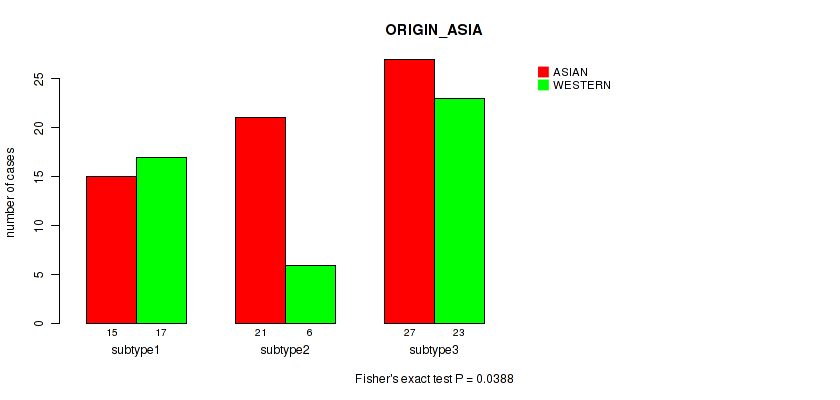
Clustering Approach #2: 'LINCRNA CHIERARCHICAL'

Table S19. Description of clustering approach #2: 'LINCRNA CHIERARCHICAL'

Cluster Labels	1	2	3
Number of samples	33	30	48

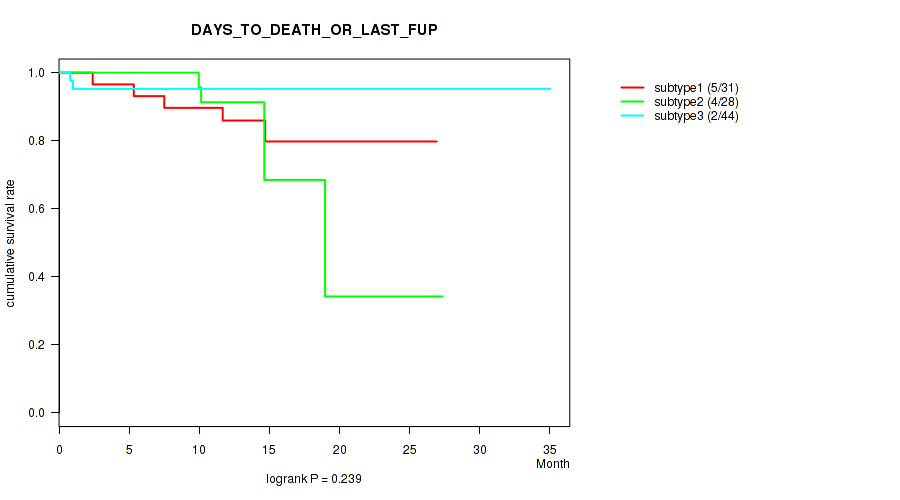
'LINCRNA CHIERARCHICAL' versus 'DAYS_TO_DEATH_OR_LAST_FUP'

P value = 0.239 (logrank test), Q value = 0.39

Table S20. Clustering Approach #2: 'LINCRNA CHIERARCHICAL' versus Clinical Feature #1: 'DAYS_TO_DEATH_OR_LAST_FUP'

	nPatients	nDeath	Duration Range (Median), Month
ALL	111	11	0.2 - 35.0 (13.1)
subtype1	31	5	1.4 - 26.9 (14.1)
subtype2	28	4	0.2 - 27.4 (12.7)
subtype3	44	2	0.5 - 35.0 (12.2)

Figure S18. Get High-res Image Clustering Approach #2: 'LINCRNA CHIERARCHICAL' versus Clinical Feature #1: 'DAYS_TO_DEATH_OR_LAST_FUP'

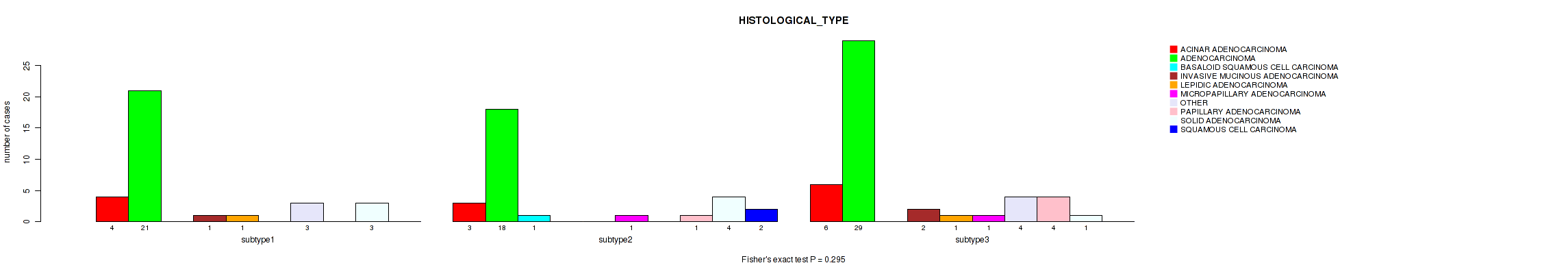
'LINCRNA CHIERARCHICAL' versus 'HISTOLOGICAL_TYPE'

P value = 0.295 (Fisher's exact test), Q value = 0.44

Table S21. Clustering Approach #2: 'LINCRNA CHIERARCHICAL' versus Clinical Feature #2: 'HISTOLOGICAL_TYPE'

nPatients	ACINAR ADENOCARCINOMA	ADENOCARCINOMA	BASALOID SQUAMOUS CELL CARCINOMA	INVASIVE MUCINOUS ADENOCARCINOMA	LEPIDIC ADENOCARCINOMA	MICROPAPILLARY ADENOCARCINOMA	OTHER	PAPILLARY ADENOCARCINOMA	SOLID ADENOCARCINOMA	SQUAMOUS CELL CARCINOMA
ALL	13	68	1	3	2	2	7	5	8	2
subtype1	4	21	0	1	1	0	3	0	3	0
subtype2	3	18	1	0	0	1	0	1	4	2
subtype3	6	29	0	2	1	1	4	4	1	0

Figure S19. Get High-res Image Clustering Approach #2: 'LINCRNA CHIERARCHICAL' versus Clinical Feature #2: 'HISTOLOGICAL_TYPE'

'LINCRNA CHIERARCHICAL' versus 'HISTOLOGIC_GRADE'

P value = 0.00879 (Fisher's exact test), Q value = 0.046

Table S22. Clustering Approach #2: 'LINCRNA CHIERARCHICAL' versus Clinical Feature #3: 'HISTOLOGIC_GRADE'

nPatients	G1	G2	G3	G4	GX
ALL	8	65	31	1	6
subtype1	2	24	5	0	2
subtype2	0	12	16	0	2
subtype3	6	29	10	1	2

Figure S20. Get High-res Image Clustering Approach #2: 'LINCRNA CHIERARCHICAL' versus Clinical Feature #3: 'HISTOLOGIC_GRADE'

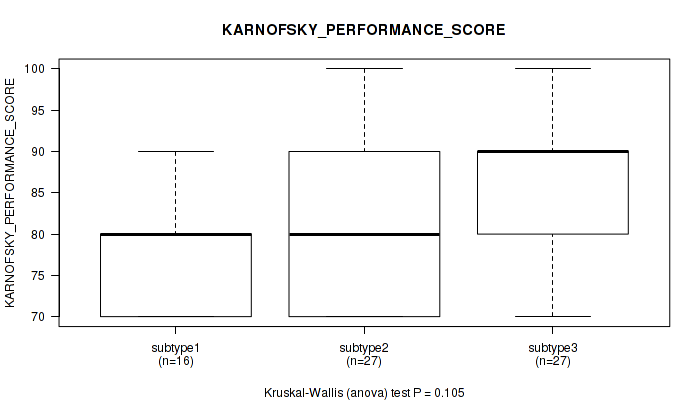
'LINCRNA CHIERARCHICAL' versus 'KARNOFSKY_PERFORMANCE_SCORE'

P value = 0.105 (Kruskal-Wallis (anova)), Q value = 0.24

Table S23. Clustering Approach #2: 'LINCRNA CHIERARCHICAL' versus Clinical Feature #4: 'KARNOFSKY_PERFORMANCE_SCORE'

	nPatients	Mean (Std.Dev)
ALL	70	81.7 (9.0)
subtype1	16	78.8 (7.2)
subtype2	27	80.7 (9.2)
subtype3	27	84.4 (9.3)

Figure S21. Get High-res Image Clustering Approach #2: 'LINCRNA CHIERARCHICAL' versus Clinical Feature #4: 'KARNOFSKY_PERFORMANCE_SCORE'

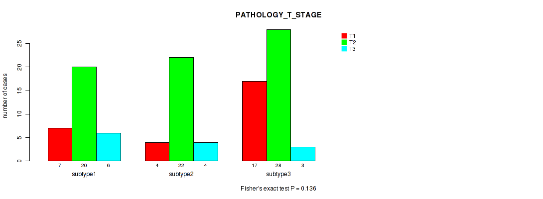
'LINCRNA CHIERARCHICAL' versus 'PATHOLOGY_T_STAGE'

P value = 0.136 (Kruskal-Wallis (anova)), Q value = 0.27

Table S24. Clustering Approach #2: 'LINCRNA CHIERARCHICAL' versus Clinical Feature #5: 'PATHOLOGY_T_STAGE'

	T1	T2	T3
ALL	28	70	13
subtype1	7	20	6
subtype2	4	22	4
subtype3	17	28	3

Figure S22. Get High-res Image Clustering Approach #2: 'LINCRNA CHIERARCHICAL' versus Clinical Feature #5: 'PATHOLOGY_T_STAGE'

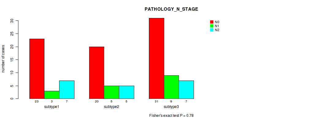
'LINCRNA CHIERARCHICAL' versus 'PATHOLOGY_N_STAGE'

P value = 0.78 (Kruskal-Wallis (anova)), Q value = 0.91

Table S25. Clustering Approach #2: 'LINCRNA CHIERARCHICAL' versus Clinical Feature #6: 'PATHOLOGY_N_STAGE'

	N0	N1	N2
ALL	74	17	19
subtype1	23	3	7
subtype2	20	5	5
subtype3	31	9	7

Figure S23. Get High-res Image Clustering Approach #2: 'LINCRNA CHIERARCHICAL' versus Clinical Feature #6: 'PATHOLOGY_N_STAGE'

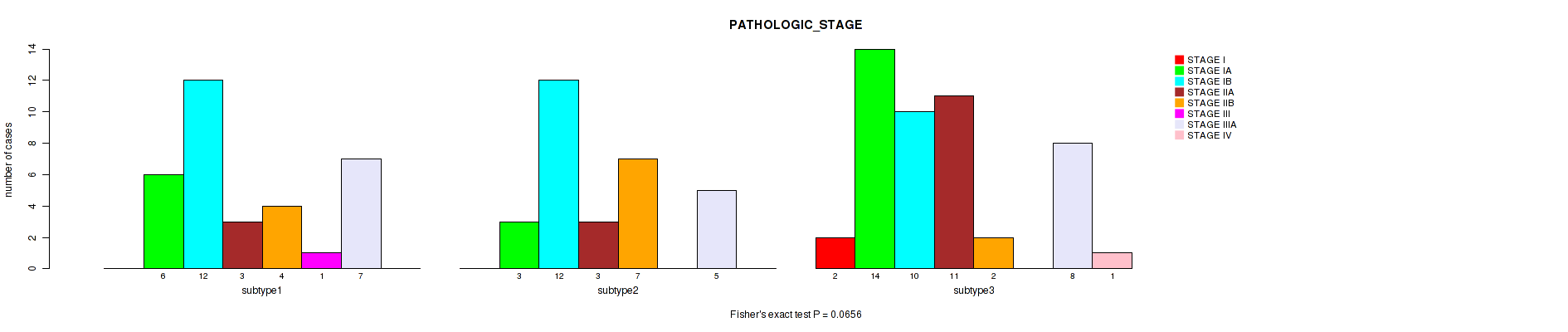
'LINCRNA CHIERARCHICAL' versus 'PATHOLOGIC_STAGE'

P value = 0.0656 (Fisher's exact test), Q value = 0.16

Table S26. Clustering Approach #2: 'LINCRNA CHIERARCHICAL' versus Clinical Feature #7: 'PATHOLOGIC_STAGE'

nPatients	STAGE I	STAGE IA	STAGE IB	STAGE IIA	STAGE IIB	STAGE III	STAGE IIIA	STAGE IV
ALL	2	23	34	17	13	1	20	1
subtype1	0	6	12	3	4	1	7	0
subtype2	0	3	12	3	7	0	5	0
subtype3	2	14	10	11	2	0	8	1

Figure S24. Get High-res Image Clustering Approach #2: 'LINCRNA CHIERARCHICAL' versus Clinical Feature #7: 'PATHOLOGIC_STAGE'

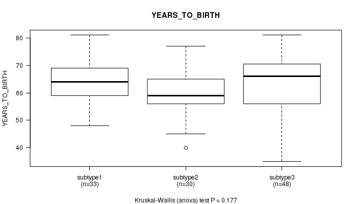
'LINCRNA CHIERARCHICAL' versus 'YEARS_TO_BIRTH'

P value = 0.177 (Kruskal-Wallis (anova)), Q value = 0.32

Table S27. Clustering Approach #2: 'LINCRNA CHIERARCHICAL' versus Clinical Feature #8: 'YEARS_TO_BIRTH'

	nPatients	Mean (Std.Dev)
ALL	111	62.6 (9.6)
subtype1	33	64.4 (7.8)
subtype2	30	60.3 (8.4)
subtype3	48	62.7 (11.2)

Figure S25. Get High-res Image Clustering Approach #2: 'LINCRNA CHIERARCHICAL' versus Clinical Feature #8: 'YEARS_TO_BIRTH'

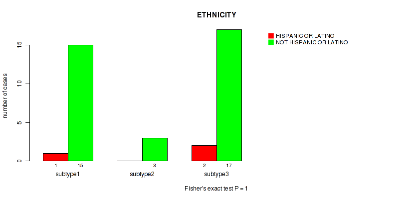
'LINCRNA CHIERARCHICAL' versus 'ETHNICITY'

P value = 1 (Fisher's exact test), Q value = 1

Table S28. Clustering Approach #2: 'LINCRNA CHIERARCHICAL' versus Clinical Feature #9: 'ETHNICITY'

nPatients	HISPANIC OR LATINO	NOT HISPANIC OR LATINO
ALL	3	35
subtype1	1	15
subtype2	0	3
subtype3	2	17

Figure S26. Get High-res Image Clustering Approach #2: 'LINCRNA CHIERARCHICAL' versus Clinical Feature #9: 'ETHNICITY'

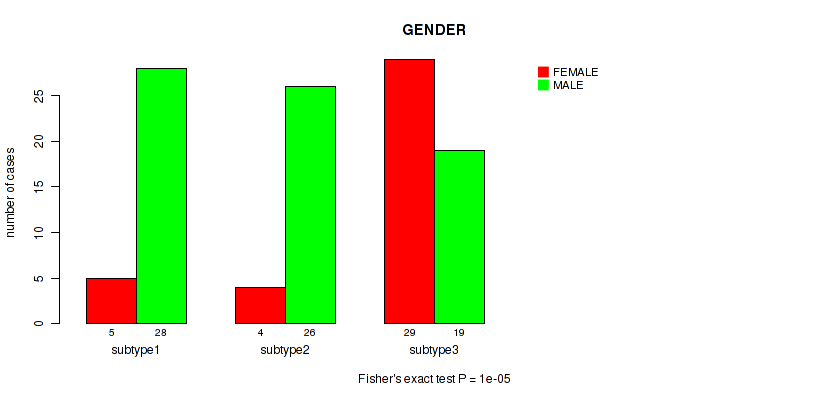
'LINCRNA CHIERARCHICAL' versus 'GENDER'

P value = 1e-05 (Fisher's exact test), Q value = 0.00034

Table S29. Clustering Approach #2: 'LINCRNA CHIERARCHICAL' versus Clinical Feature #10: 'GENDER'

nPatients	FEMALE	MALE
ALL	38	73
subtype1	5	28
subtype2	4	26
subtype3	29	19

Figure S27. Get High-res Image Clustering Approach #2: 'LINCRNA CHIERARCHICAL' versus Clinical Feature #10: 'GENDER'

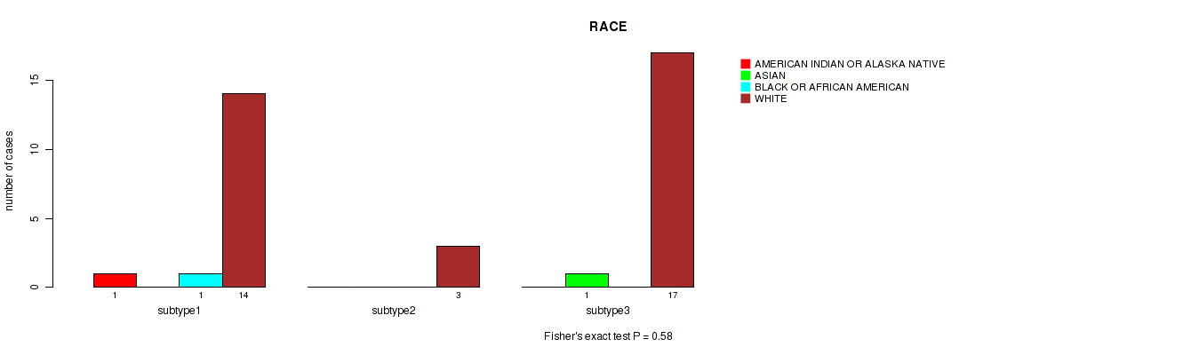
'LINCRNA CHIERARCHICAL' versus 'RACE'

P value = 0.58 (Fisher's exact test), Q value = 0.76

Table S30. Clustering Approach #2: 'LINCRNA CHIERARCHICAL' versus Clinical Feature #11: 'RACE'

nPatients	AMERICAN INDIAN OR ALASKA NATIVE	ASIAN	BLACK OR AFRICAN AMERICAN	WHITE
ALL	1	1	1	34
subtype1	1	0	1	14
subtype2	0	0	0	3
subtype3	0	1	0	17

Figure S28. Get High-res Image Clustering Approach #2: 'LINCRNA CHIERARCHICAL' versus Clinical Feature #11: 'RACE'

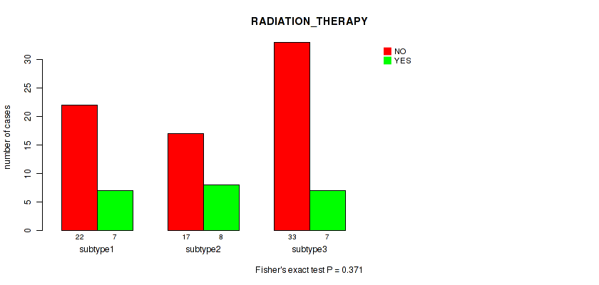
'LINCRNA CHIERARCHICAL' versus 'RADIATION_THERAPY'

P value = 0.371 (Fisher's exact test), Q value = 0.53

Table S31. Clustering Approach #2: 'LINCRNA CHIERARCHICAL' versus Clinical Feature #12: 'RADIATION_THERAPY'

nPatients	NO	YES
ALL	72	22
subtype1	22	7
subtype2	17	8
subtype3	33	7

Figure S29. Get High-res Image Clustering Approach #2: 'LINCRNA CHIERARCHICAL' versus Clinical Feature #12: 'RADIATION_THERAPY'

'LINCRNA CHIERARCHICAL' versus 'BMI'

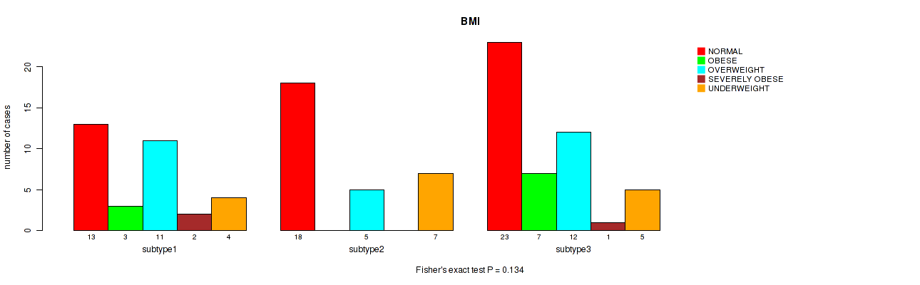
P value = 0.134 (Fisher's exact test), Q value = 0.27

Table S32. Clustering Approach #2: 'LINCRNA CHIERARCHICAL' versus Clinical Feature #13: 'BMI'

nPatients	NORMAL	OBESE	OVERWEIGHT	SEVERELY OBESE	UNDERWEIGHT
ALL	54	10	28	3	16
subtype1	13	3	11	2	4
subtype2	18	0	5	0	7
subtype3	23	7	12	1	5

Figure S30. Get High-res Image Clustering Approach #2: 'LINCRNA CHIERARCHICAL' versus Clinical Feature #13: 'BMI'

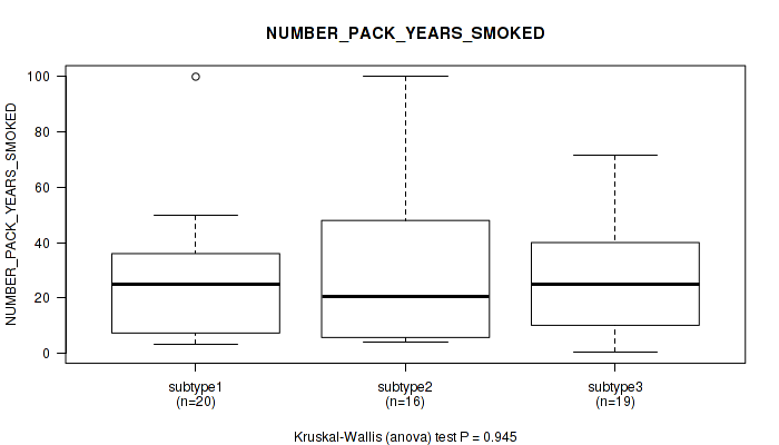
'LINCRNA CHIERARCHICAL' versus 'NUMBER_PACK_YEARS_SMOKED'

P value = 0.945 (Kruskal-Wallis (anova)), Q value = 1

Table S33. Clustering Approach #2: 'LINCRNA CHIERARCHICAL' versus Clinical Feature #14: 'NUMBER_PACK_YEARS_SMOKED'

	nPatients	Mean (Std.Dev)
ALL	55	27.4 (23.4)
subtype1	20	26.3 (23.2)
subtype2	16	28.6 (28.0)
subtype3	19	27.5 (20.4)

Figure S31. Get High-res Image Clustering Approach #2: 'LINCRNA CHIERARCHICAL' versus Clinical Feature #14: 'NUMBER_PACK_YEARS_SMOKED'

'LINCRNA CHIERARCHICAL' versus 'SMOKER'

P value = 0.0245 (Fisher's exact test), Q value = 0.093

Table S34. Clustering Approach #2: 'LINCRNA CHIERARCHICAL' versus Clinical Feature #15: 'SMOKER'

nPatients	NON-SMOKER	SMOKER
ALL	46	62
subtype1	8	25
subtype2	13	16
subtype3	25	21

Figure S32. Get High-res Image Clustering Approach #2: 'LINCRNA CHIERARCHICAL' versus Clinical Feature #15: 'SMOKER'

'LINCRNA CHIERARCHICAL' versus 'COUNTRY_OF_ORIGIN'

P value = 0.00014 (Fisher's exact test), Q value = 0.0016

Table S35. Clustering Approach #2: 'LINCRNA CHIERARCHICAL' versus Clinical Feature #16: 'COUNTRY_OF_ORIGIN'

nPatients	BULGARIA	CANADA	CHINA	JAMAICA	MEXICO	POLAND	RUSSIA	UKRAINE	UNITED STATES	VIETNAM
ALL	2	1	18	1	2	2	1	3	34	45
subtype1	1	0	0	1	1	0	1	2	14	13
subtype2	1	0	5	0	0	1	0	1	3	19
subtype3	0	1	13	0	1	1	0	0	17	13

Figure S33. Get High-res Image Clustering Approach #2: 'LINCRNA CHIERARCHICAL' versus Clinical Feature #16: 'COUNTRY_OF_ORIGIN'

'LINCRNA CHIERARCHICAL' versus 'ORIGIN_ASIA'

P value = 0.00495 (Fisher's exact test), Q value = 0.034

Table S36. Clustering Approach #2: 'LINCRNA CHIERARCHICAL' versus Clinical Feature #17: 'ORIGIN_ASIA'

nPatients	ASIAN	WESTERN
ALL	63	46
subtype1	13	20
subtype2	24	6
subtype3	26	20

Figure S34. Get High-res Image Clustering Approach #2: 'LINCRNA CHIERARCHICAL' versus Clinical Feature #17: 'ORIGIN_ASIA'

Methods & Data

Input

Cluster data file = /cromwell_root/fc-e7058367-eaa6-44b5-aab5-1ec08acf146a/69dd18b3-97fe-4143-b0f4-32e5d55e929d/aggregate_clusters_workflow/d44c315a-761b-4b72-be1f-cb969be36102/call-aggregate_clusters/CPTAC3-LUAD-TP.mergedcluster.txt
Clinical data file = /cromwell_root/fc-e7058367-eaa6-44b5-aab5-1ec08acf146a/39eab10a-1791-41cf-866c-13e6472ce02e/normalize_clinical_cptac/df4eac3a-77b6-4ce7-961f-e1027c1ad609/call-normalize_clinical_cptac_task_1/CPTAC3-LUAD-TP.clin.merged.picked.txt
Number of patients = 111
Number of clustering approaches = 2
Number of selected clinical features = 17
Exclude small clusters that include fewer than K patients, K = 3

Clustering approaches

Consensus hierarchical clustering

Resampling-based clustering method (Monti et al. 2003)

Survival analysis

For survival clinical features, the Kaplan-Meier survival curves of tumors with and without gene mutations were plotted and the statistical significance P values were estimated by logrank test (Bland and Altman 2004) using the 'survdiff' function in R

Fisher's exact test

For binary clinical features, two-tailed Fisher's exact tests (Fisher 1922) were used to estimate the P values using the 'fisher.test' function in R

Q value calculation

For multiple hypothesis correction, Q value is the False Discovery Rate (FDR) analogue of the P value (Benjamini and Hochberg 1995), defined as the minimum FDR at which the test may be called significant. We used the 'Benjamini and Hochberg' method of 'p.adjust' function in R to convert P values into Q values.

References

[1] Monti et al., Consensus Clustering: A Resampling-Based Method for Class Discovery and Visualization of Gene Expression Microarray Data, Machine Learning 52(1):91-118 (2003)

[2] Bland and Altman, Statistics notes: The logrank test, BMJ 328(7447):1073 (2004)

[3] Fisher, R.A., On the interpretation of chi-square from contingency tables, and the calculation of P, Journal of the Royal Statistical Society 85(1):87-94 (1922)

[4] Benjamini and Hochberg, Controlling the false discovery rate: a practical and powerful approach to multiple testing, Journal of the Royal Statistical Society Series B 59:289-300 (1995)

Made with Nozzle