Correlation between aggregated molecular cancer subtypes and selected clinical features

Uterine Corpus Endometrioid Carcinoma (Primary solid tumor)

04 October 2018 | None

Maintainer Information

Maintained by Broad Institute GDAC (Broad Institute of MIT & Harvard)

Overview

Introduction

This pipeline computes the correlation between cancer subtypes identified by different molecular patterns and selected clinical features.

Summary

Testing the association between subtypes identified by 3 different clustering approaches and 17 clinical features across 100 patients, 3 significant findings detected with P value < 0.05 and Q value < 0.25.

Consensus hierarchical clustering analysis on array-based mRNA expression data identified 5 subtypes that do not correlate to any clinical features.
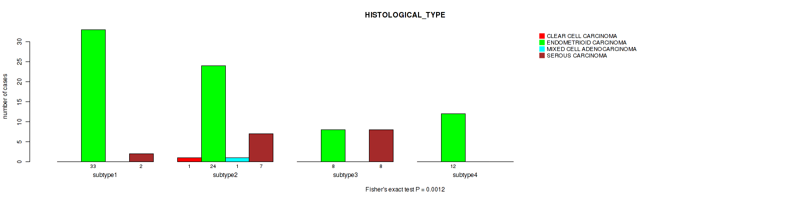
CNMF clustering analysis on methylation data identified 4 subtypes that correlate to 'HISTOLOGICAL_TYPE'.
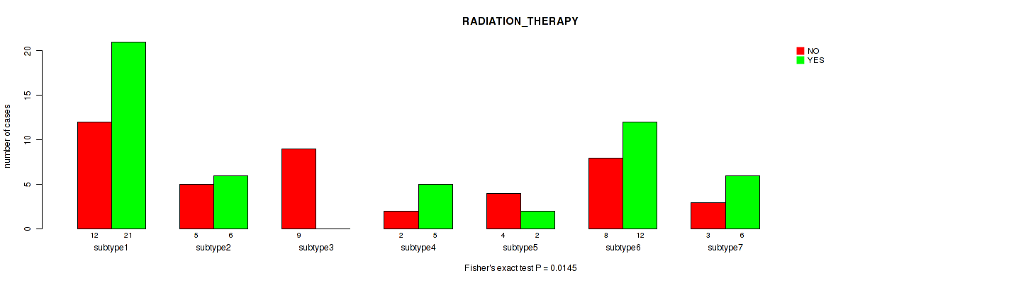
7 subtypes identified in current cancer cohort by 'METHYLATION CHIERARCHICAL'. These subtypes correlate to 'HISTOLOGICAL_TYPE' and 'RADIATION_THERAPY'.

Results

Overview of the results

Table 1. Get Full Table Overview of the association between subtypes identified by 3 different clustering approaches and 17 clinical features. Shown in the table are P values (Q values). Thresholded by P value < 0.05 and Q value < 0.25, 3 significant findings detected.


Clinical Features	Statistical Tests	mRNA cHierClus subtypes	Methylation CNMF subtypes	METHYLATION CHIERARCHICAL
DAYS TO DEATH OR LAST FUP	logrank test	0.412 (0.83)	0.818 (0.909)	0.585 (0.847)
HISTOLOGICAL TYPE	Fisher's exact test	0.713 (0.909)	0.0012 (0.0306)	0.00011 (0.00561)
FIGO GRADE	Fisher's exact test	0.315 (0.81)	0.027 (0.344)	0.472 (0.83)
KARNOFSKY PERFORMANCE SCORE	Kruskal-Wallis (anova)	0.526 (0.838)	0.0369 (0.377)	0.133 (0.519)
MSI	Fisher's exact test	0.574 (0.847)	1 (1.00)	0.479 (0.83)
PATHOLOGY T STAGE	Fisher's exact test	0.108 (0.459)	0.148 (0.519)	0.584 (0.847)
PATHOLOGY N STAGE	Fisher's exact test	0.386 (0.83)	0.818 (0.909)	0.45 (0.83)
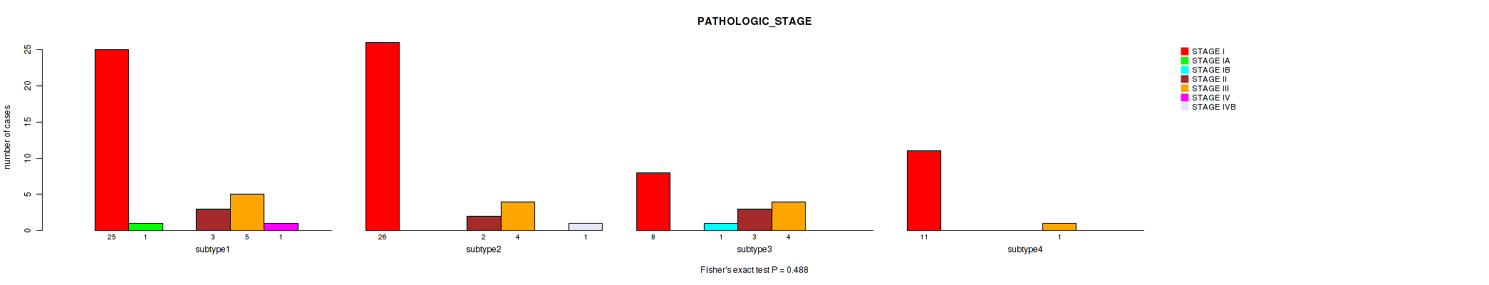
PATHOLOGIC STAGE	Fisher's exact test	0.36 (0.83)	0.488 (0.83)	0.484 (0.83)
YEARS TO BIRTH	Kruskal-Wallis (anova)	0.517 (0.838)	0.82 (0.909)	0.47 (0.83)
ETHNICITY	Fisher's exact test	0.28 (0.792)	0.0768 (0.426)	0.844 (0.909)
RACE	Fisher's exact test	0.849 (0.909)	0.364 (0.83)	0.266 (0.792)
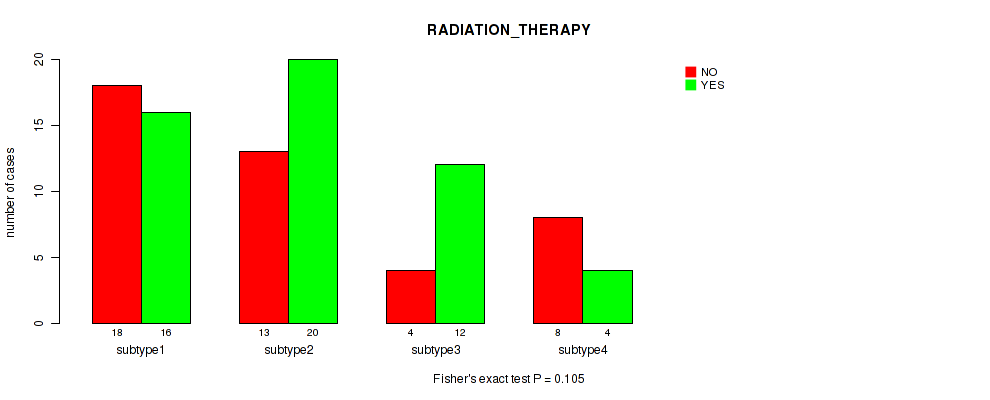
RADIATION THERAPY	Fisher's exact test	0.919 (0.956)	0.105 (0.459)	0.0145 (0.246)
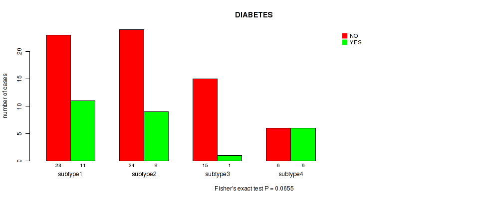
DIABETES	Fisher's exact test	0.83 (0.909)	0.0655 (0.422)	0.67 (0.909)
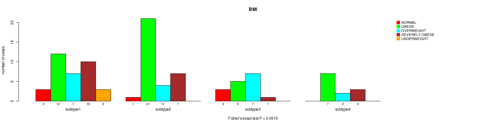
BMI	Fisher's exact test	0.0661 (0.422)	0.0515 (0.422)	0.598 (0.847)
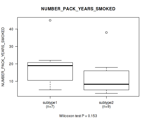
NUMBER PACK YEARS SMOKED	Kruskal-Wallis (anova)	0.318 (0.81)	0.153 (0.519)	0.0835 (0.426)
SMOKER	Fisher's exact test	0.855 (0.909)	0.26 (0.792)	0.734 (0.909)
COUNTRY OF ORIGIN	Fisher's exact test	0.728 (0.909)	0.679 (0.909)	0.947 (0.966)

Clustering Approach #1: 'mRNA cHierClus subtypes'

Table S1. Description of clustering approach #1: 'mRNA cHierClus subtypes'

Cluster Labels	1	2	3	4	5
Number of samples	28	20	11	20	21

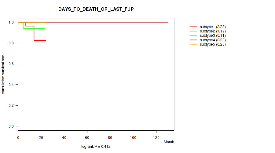
'mRNA cHierClus subtypes' versus 'DAYS_TO_DEATH_OR_LAST_FUP'

P value = 0.412 (logrank test), Q value = 0.83

Table S2. Clustering Approach #1: 'mRNA cHierClus subtypes' versus Clinical Feature #1: 'DAYS_TO_DEATH_OR_LAST_FUP'

	nPatients	nDeath	Duration Range (Median), Month
ALL	99	3	0.0 - 130.4 (11.6)
subtype1	28	2	5.4 - 24.3 (11.2)
subtype2	19	1	0.0 - 23.3 (10.8)
subtype3	11	0	1.9 - 23.5 (14.0)
subtype4	20	0	6.0 - 130.4 (12.6)
subtype5	20	0	6.6 - 24.8 (11.8)

Figure S1. Get High-res Image Clustering Approach #1: 'mRNA cHierClus subtypes' versus Clinical Feature #1: 'DAYS_TO_DEATH_OR_LAST_FUP'

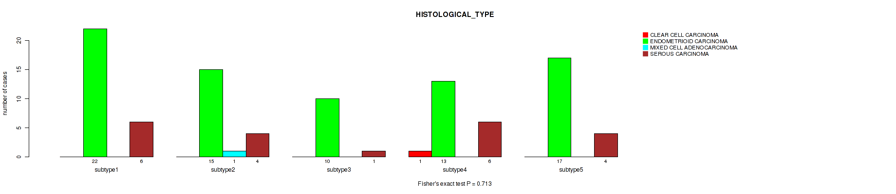
'mRNA cHierClus subtypes' versus 'HISTOLOGICAL_TYPE'

P value = 0.713 (Fisher's exact test), Q value = 0.91

Table S3. Clustering Approach #1: 'mRNA cHierClus subtypes' versus Clinical Feature #2: 'HISTOLOGICAL_TYPE'

nPatients	CLEAR CELL CARCINOMA	ENDOMETRIOID CARCINOMA	MIXED CELL ADENOCARCINOMA	SEROUS CARCINOMA
ALL	1	77	1	21
subtype1	0	22	0	6
subtype2	0	15	1	4
subtype3	0	10	0	1
subtype4	1	13	0	6
subtype5	0	17	0	4

Figure S2. Get High-res Image Clustering Approach #1: 'mRNA cHierClus subtypes' versus Clinical Feature #2: 'HISTOLOGICAL_TYPE'

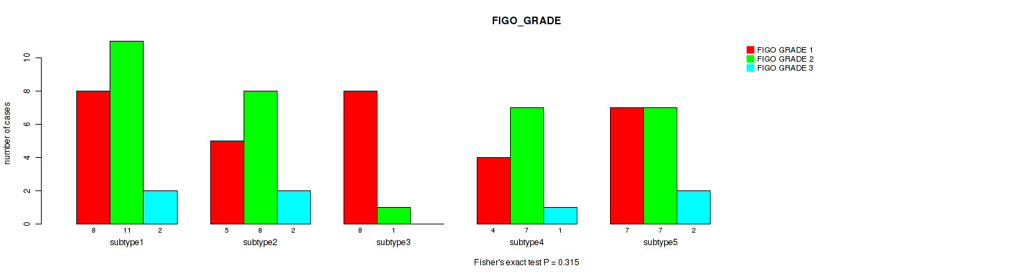
'mRNA cHierClus subtypes' versus 'FIGO_GRADE'

P value = 0.315 (Fisher's exact test), Q value = 0.81

Table S4. Clustering Approach #1: 'mRNA cHierClus subtypes' versus Clinical Feature #3: 'FIGO_GRADE'

nPatients	FIGO GRADE 1	FIGO GRADE 2	FIGO GRADE 3
ALL	32	34	7
subtype1	8	11	2
subtype2	5	8	2
subtype3	8	1	0
subtype4	4	7	1
subtype5	7	7	2

Figure S3. Get High-res Image Clustering Approach #1: 'mRNA cHierClus subtypes' versus Clinical Feature #3: 'FIGO_GRADE'

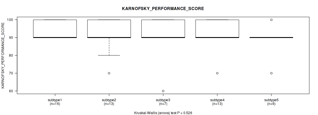
'mRNA cHierClus subtypes' versus 'KARNOFSKY_PERFORMANCE_SCORE'

P value = 0.526 (Kruskal-Wallis (anova)), Q value = 0.84

Table S5. Clustering Approach #1: 'mRNA cHierClus subtypes' versus Clinical Feature #4: 'KARNOFSKY_PERFORMANCE_SCORE'

	nPatients	Mean (Std.Dev)
ALL	58	91.9 (8.5)
subtype1	16	94.4 (5.1)
subtype2	13	92.3 (9.3)
subtype3	7	90.0 (14.1)
subtype4	13	91.5 (8.0)
subtype5	9	88.9 (7.8)

Figure S4. Get High-res Image Clustering Approach #1: 'mRNA cHierClus subtypes' versus Clinical Feature #4: 'KARNOFSKY_PERFORMANCE_SCORE'

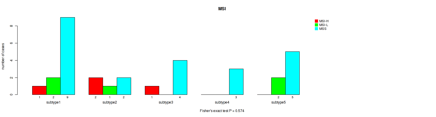
'mRNA cHierClus subtypes' versus 'MSI'

P value = 0.574 (Fisher's exact test), Q value = 0.85

Table S6. Clustering Approach #1: 'mRNA cHierClus subtypes' versus Clinical Feature #5: 'MSI'

nPatients	MSI-H	MSI-L	MSS
ALL	4	5	23
subtype1	1	2	9
subtype2	2	1	2
subtype3	1	0	4
subtype4	0	0	3
subtype5	0	2	5

Figure S5. Get High-res Image Clustering Approach #1: 'mRNA cHierClus subtypes' versus Clinical Feature #5: 'MSI'

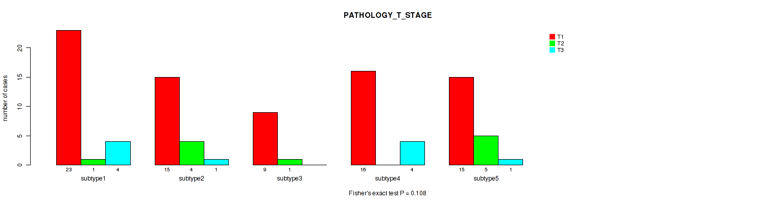
'mRNA cHierClus subtypes' versus 'PATHOLOGY_T_STAGE'

P value = 0.108 (Kruskal-Wallis (anova)), Q value = 0.46

Table S7. Clustering Approach #1: 'mRNA cHierClus subtypes' versus Clinical Feature #6: 'PATHOLOGY_T_STAGE'

	T1	T2	T3
ALL	78	11	10
subtype1	23	1	4
subtype2	15	4	1
subtype3	9	1	0
subtype4	16	0	4
subtype5	15	5	1

Figure S6. Get High-res Image Clustering Approach #1: 'mRNA cHierClus subtypes' versus Clinical Feature #6: 'PATHOLOGY_T_STAGE'

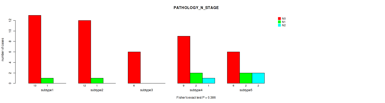
'mRNA cHierClus subtypes' versus 'PATHOLOGY_N_STAGE'

P value = 0.386 (Kruskal-Wallis (anova)), Q value = 0.83

Table S8. Clustering Approach #1: 'mRNA cHierClus subtypes' versus Clinical Feature #7: 'PATHOLOGY_N_STAGE'

	N0	N1	N2
ALL	46	6	3
subtype1	13	1	0
subtype2	12	1	0
subtype3	6	0	0
subtype4	9	2	1
subtype5	6	2	2

Figure S7. Get High-res Image Clustering Approach #1: 'mRNA cHierClus subtypes' versus Clinical Feature #7: 'PATHOLOGY_N_STAGE'

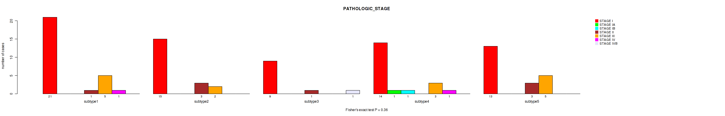
'mRNA cHierClus subtypes' versus 'PATHOLOGIC_STAGE'

P value = 0.36 (Fisher's exact test), Q value = 0.83

Table S9. Clustering Approach #1: 'mRNA cHierClus subtypes' versus Clinical Feature #8: 'PATHOLOGIC_STAGE'

nPatients	STAGE I	STAGE IA	STAGE IB	STAGE II	STAGE III	STAGE IV	STAGE IVB
ALL	72	1	1	8	15	2	1
subtype1	21	0	0	1	5	1	0
subtype2	15	0	0	3	2	0	0
subtype3	9	0	0	1	0	0	1
subtype4	14	1	1	0	3	1	0
subtype5	13	0	0	3	5	0	0

Figure S8. Get High-res Image Clustering Approach #1: 'mRNA cHierClus subtypes' versus Clinical Feature #8: 'PATHOLOGIC_STAGE'

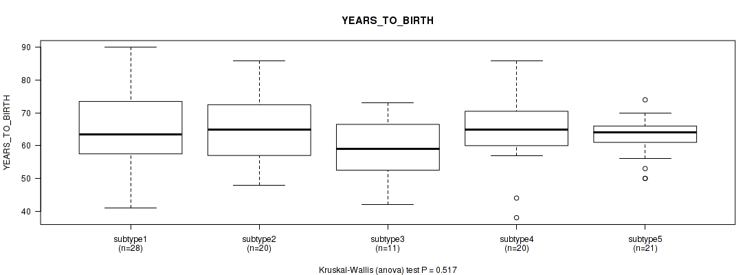
'mRNA cHierClus subtypes' versus 'YEARS_TO_BIRTH'

P value = 0.517 (Kruskal-Wallis (anova)), Q value = 0.84

Table S10. Clustering Approach #1: 'mRNA cHierClus subtypes' versus Clinical Feature #9: 'YEARS_TO_BIRTH'

	nPatients	Mean (Std.Dev)
ALL	100	63.6 (10.1)
subtype1	28	64.6 (12.0)
subtype2	20	65.0 (9.6)
subtype3	11	58.7 (10.2)
subtype4	20	64.3 (10.7)
subtype5	21	62.6 (6.2)

Figure S9. Get High-res Image Clustering Approach #1: 'mRNA cHierClus subtypes' versus Clinical Feature #9: 'YEARS_TO_BIRTH'

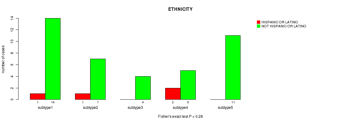
'mRNA cHierClus subtypes' versus 'ETHNICITY'

P value = 0.28 (Fisher's exact test), Q value = 0.79

Table S11. Clustering Approach #1: 'mRNA cHierClus subtypes' versus Clinical Feature #10: 'ETHNICITY'

nPatients	HISPANIC OR LATINO	NOT HISPANIC OR LATINO
ALL	4	41
subtype1	1	14
subtype2	1	7
subtype3	0	4
subtype4	2	5
subtype5	0	11

Figure S10. Get High-res Image Clustering Approach #1: 'mRNA cHierClus subtypes' versus Clinical Feature #10: 'ETHNICITY'

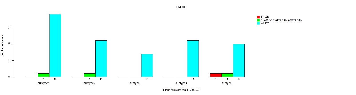
'mRNA cHierClus subtypes' versus 'RACE'

P value = 0.849 (Fisher's exact test), Q value = 0.91

Table S12. Clustering Approach #1: 'mRNA cHierClus subtypes' versus Clinical Feature #11: 'RACE'

nPatients	ASIAN	BLACK OR AFRICAN AMERICAN	WHITE
ALL	1	3	58
subtype1	0	1	19
subtype2	0	1	11
subtype3	0	0	7
subtype4	0	0	11
subtype5	1	1	10

Figure S11. Get High-res Image Clustering Approach #1: 'mRNA cHierClus subtypes' versus Clinical Feature #11: 'RACE'

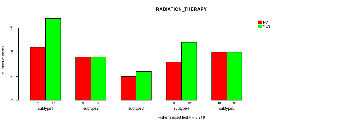
'mRNA cHierClus subtypes' versus 'RADIATION_THERAPY'

P value = 0.919 (Fisher's exact test), Q value = 0.96

Table S13. Clustering Approach #1: 'mRNA cHierClus subtypes' versus Clinical Feature #12: 'RADIATION_THERAPY'

nPatients	NO	YES
ALL	43	54
subtype1	11	17
subtype2	9	9
subtype3	5	6
subtype4	8	12
subtype5	10	10

Figure S12. Get High-res Image Clustering Approach #1: 'mRNA cHierClus subtypes' versus Clinical Feature #12: 'RADIATION_THERAPY'

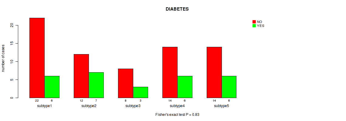
'mRNA cHierClus subtypes' versus 'DIABETES'

P value = 0.83 (Fisher's exact test), Q value = 0.91

Table S14. Clustering Approach #1: 'mRNA cHierClus subtypes' versus Clinical Feature #13: 'DIABETES'

nPatients	NO	YES
ALL	70	28
subtype1	22	6
subtype2	12	7
subtype3	8	3
subtype4	14	6
subtype5	14	6

Figure S13. Get High-res Image Clustering Approach #1: 'mRNA cHierClus subtypes' versus Clinical Feature #13: 'DIABETES'

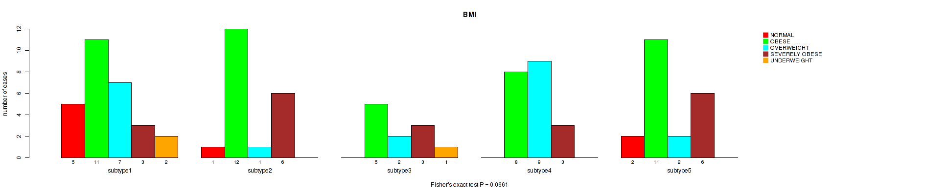
'mRNA cHierClus subtypes' versus 'BMI'

P value = 0.0661 (Fisher's exact test), Q value = 0.42

Table S15. Clustering Approach #1: 'mRNA cHierClus subtypes' versus Clinical Feature #14: 'BMI'

nPatients	NORMAL	OBESE	OVERWEIGHT	SEVERELY OBESE	UNDERWEIGHT
ALL	8	47	21	21	3
subtype1	5	11	7	3	2
subtype2	1	12	1	6	0
subtype3	0	5	2	3	1
subtype4	0	8	9	3	0
subtype5	2	11	2	6	0

Figure S14. Get High-res Image Clustering Approach #1: 'mRNA cHierClus subtypes' versus Clinical Feature #14: 'BMI'

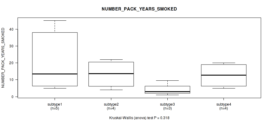
'mRNA cHierClus subtypes' versus 'NUMBER_PACK_YEARS_SMOKED'

P value = 0.318 (Kruskal-Wallis (anova)), Q value = 0.81

Table S16. Clustering Approach #1: 'mRNA cHierClus subtypes' versus Clinical Feature #15: 'NUMBER_PACK_YEARS_SMOKED'

	nPatients	Mean (Std.Dev)
ALL	18	14.5 (11.9)
subtype1	5	21.6 (18.7)
subtype2	4	13.3 (8.6)
subtype3	3	4.5 (4.4)
subtype4	4	12.6 (7.5)
subtype5	2	17.8 (2.5)

Figure S15. Get High-res Image Clustering Approach #1: 'mRNA cHierClus subtypes' versus Clinical Feature #15: 'NUMBER_PACK_YEARS_SMOKED'

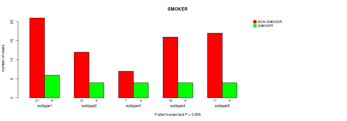
'mRNA cHierClus subtypes' versus 'SMOKER'

P value = 0.855 (Fisher's exact test), Q value = 0.91

Table S17. Clustering Approach #1: 'mRNA cHierClus subtypes' versus Clinical Feature #16: 'SMOKER'

nPatients	NON-SMOKER	SMOKER
ALL	73	22
subtype1	21	6
subtype2	12	4
subtype3	7	4
subtype4	16	4
subtype5	17	4

Figure S16. Get High-res Image Clustering Approach #1: 'mRNA cHierClus subtypes' versus Clinical Feature #16: 'SMOKER'

'mRNA cHierClus subtypes' versus 'COUNTRY_OF_ORIGIN'

P value = 0.728 (Fisher's exact test), Q value = 0.91

Table S18. Clustering Approach #1: 'mRNA cHierClus subtypes' versus Clinical Feature #17: 'COUNTRY_OF_ORIGIN'

nPatients	MEXICO	POLAND	UKRAINE	UNITED STATES
ALL	2	5	32	36
subtype1	0	0	8	12
subtype2	1	1	6	4
subtype3	0	1	3	4
subtype4	1	2	7	6
subtype5	0	1	8	10

Figure S17. Get High-res Image Clustering Approach #1: 'mRNA cHierClus subtypes' versus Clinical Feature #17: 'COUNTRY_OF_ORIGIN'

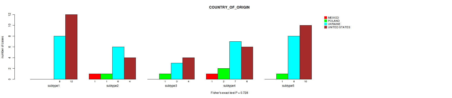
Clustering Approach #2: 'Methylation CNMF subtypes'

Table S19. Description of clustering approach #2: 'Methylation CNMF subtypes'

Cluster Labels	1	2	3	4
Number of samples	35	33	16	12

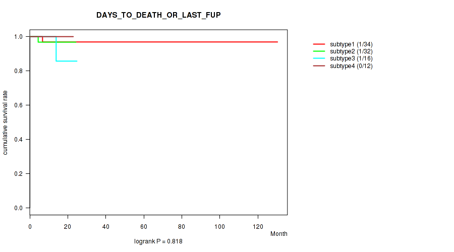
'Methylation CNMF subtypes' versus 'DAYS_TO_DEATH_OR_LAST_FUP'

P value = 0.818 (logrank test), Q value = 0.91

Table S20. Clustering Approach #2: 'Methylation CNMF subtypes' versus Clinical Feature #1: 'DAYS_TO_DEATH_OR_LAST_FUP'

	nPatients	nDeath	Duration Range (Median), Month
ALL	95	3	1.9 - 130.4 (11.6)
subtype1	34	1	6.1 - 130.4 (11.6)
subtype2	32	1	2.3 - 24.3 (10.9)
subtype3	16	1	1.9 - 24.8 (11.4)
subtype4	12	0	9.6 - 22.9 (14.5)

Figure S18. Get High-res Image Clustering Approach #2: 'Methylation CNMF subtypes' versus Clinical Feature #1: 'DAYS_TO_DEATH_OR_LAST_FUP'

'Methylation CNMF subtypes' versus 'HISTOLOGICAL_TYPE'

P value = 0.0012 (Fisher's exact test), Q value = 0.031

Table S21. Clustering Approach #2: 'Methylation CNMF subtypes' versus Clinical Feature #2: 'HISTOLOGICAL_TYPE'

nPatients	CLEAR CELL CARCINOMA	ENDOMETRIOID CARCINOMA	MIXED CELL ADENOCARCINOMA	SEROUS CARCINOMA
ALL	1	77	1	17
subtype1	0	33	0	2
subtype2	1	24	1	7
subtype3	0	8	0	8
subtype4	0	12	0	0

Figure S19. Get High-res Image Clustering Approach #2: 'Methylation CNMF subtypes' versus Clinical Feature #2: 'HISTOLOGICAL_TYPE'

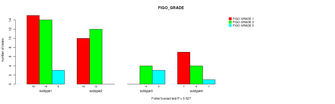
'Methylation CNMF subtypes' versus 'FIGO_GRADE'

P value = 0.027 (Fisher's exact test), Q value = 0.34

Table S22. Clustering Approach #2: 'Methylation CNMF subtypes' versus Clinical Feature #3: 'FIGO_GRADE'

nPatients	FIGO GRADE 1	FIGO GRADE 2	FIGO GRADE 3
ALL	32	34	7
subtype1	15	14	3
subtype2	10	12	0
subtype3	0	4	3
subtype4	7	4	1

Figure S20. Get High-res Image Clustering Approach #2: 'Methylation CNMF subtypes' versus Clinical Feature #3: 'FIGO_GRADE'

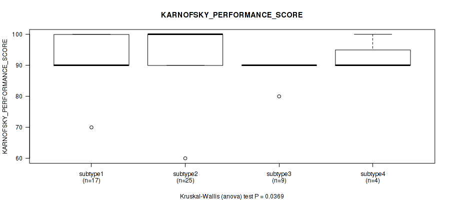
'Methylation CNMF subtypes' versus 'KARNOFSKY_PERFORMANCE_SCORE'

P value = 0.0369 (Kruskal-Wallis (anova)), Q value = 0.38

Table S23. Clustering Approach #2: 'Methylation CNMF subtypes' versus Clinical Feature #4: 'KARNOFSKY_PERFORMANCE_SCORE'

	nPatients	Mean (Std.Dev)
ALL	55	92.7 (7.6)
subtype1	17	92.4 (7.5)
subtype2	25	94.4 (8.7)
subtype3	9	88.9 (3.3)
subtype4	4	92.5 (5.0)

Figure S21. Get High-res Image Clustering Approach #2: 'Methylation CNMF subtypes' versus Clinical Feature #4: 'KARNOFSKY_PERFORMANCE_SCORE'

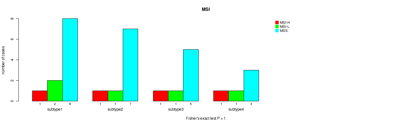
'Methylation CNMF subtypes' versus 'MSI'

P value = 1 (Fisher's exact test), Q value = 1

Table S24. Clustering Approach #2: 'Methylation CNMF subtypes' versus Clinical Feature #5: 'MSI'

nPatients	MSI-H	MSI-L	MSS
ALL	4	5	23
subtype1	1	2	8
subtype2	1	1	7
subtype3	1	1	5
subtype4	1	1	3

Figure S22. Get High-res Image Clustering Approach #2: 'Methylation CNMF subtypes' versus Clinical Feature #5: 'MSI'

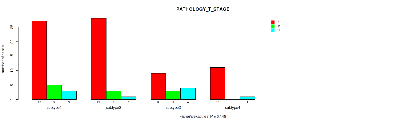
'Methylation CNMF subtypes' versus 'PATHOLOGY_T_STAGE'

P value = 0.148 (Kruskal-Wallis (anova)), Q value = 0.52

Table S25. Clustering Approach #2: 'Methylation CNMF subtypes' versus Clinical Feature #6: 'PATHOLOGY_T_STAGE'

	T1	T2	T3
ALL	75	11	9
subtype1	27	5	3
subtype2	28	3	1
subtype3	9	3	4
subtype4	11	0	1

Figure S23. Get High-res Image Clustering Approach #2: 'Methylation CNMF subtypes' versus Clinical Feature #6: 'PATHOLOGY_T_STAGE'

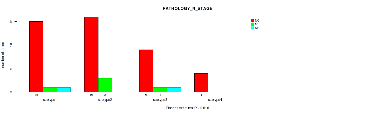
'Methylation CNMF subtypes' versus 'PATHOLOGY_N_STAGE'

P value = 0.818 (Kruskal-Wallis (anova)), Q value = 0.91

Table S26. Clustering Approach #2: 'Methylation CNMF subtypes' versus Clinical Feature #7: 'PATHOLOGY_N_STAGE'

	N0	N1	N2
ALL	44	5	2
subtype1	15	1	1
subtype2	16	3	0
subtype3	9	1	1
subtype4	4	0	0

Figure S24. Get High-res Image Clustering Approach #2: 'Methylation CNMF subtypes' versus Clinical Feature #7: 'PATHOLOGY_N_STAGE'

'Methylation CNMF subtypes' versus 'PATHOLOGIC_STAGE'

P value = 0.488 (Fisher's exact test), Q value = 0.83

Table S27. Clustering Approach #2: 'Methylation CNMF subtypes' versus Clinical Feature #8: 'PATHOLOGIC_STAGE'

nPatients	STAGE I	STAGE IA	STAGE IB	STAGE II	STAGE III	STAGE IV	STAGE IVB
ALL	70	1	1	8	14	1	1
subtype1	25	1	0	3	5	1	0
subtype2	26	0	0	2	4	0	1
subtype3	8	0	1	3	4	0	0
subtype4	11	0	0	0	1	0	0

Figure S25. Get High-res Image Clustering Approach #2: 'Methylation CNMF subtypes' versus Clinical Feature #8: 'PATHOLOGIC_STAGE'

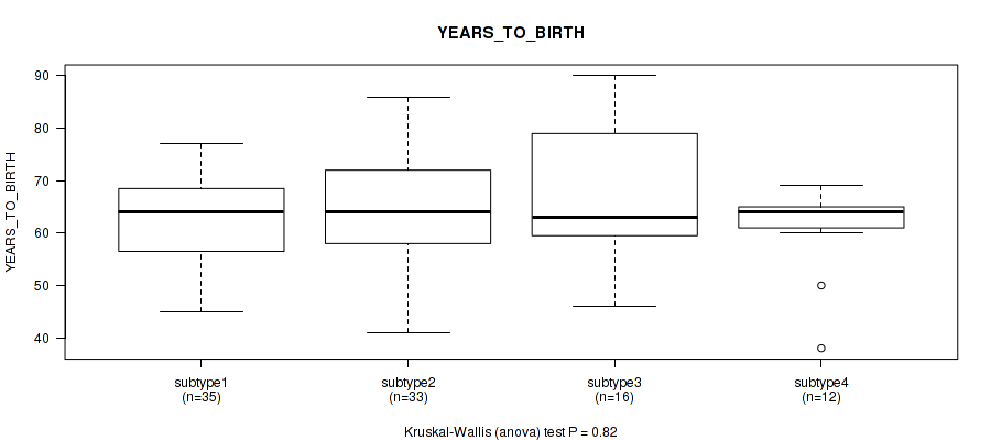
'Methylation CNMF subtypes' versus 'YEARS_TO_BIRTH'

P value = 0.82 (Kruskal-Wallis (anova)), Q value = 0.91

Table S28. Clustering Approach #2: 'Methylation CNMF subtypes' versus Clinical Feature #9: 'YEARS_TO_BIRTH'

	nPatients	Mean (Std.Dev)
ALL	96	63.5 (10.2)
subtype1	35	62.6 (8.3)
subtype2	33	63.5 (10.6)
subtype3	16	67.1 (13.4)
subtype4	12	60.9 (8.6)

Figure S26. Get High-res Image Clustering Approach #2: 'Methylation CNMF subtypes' versus Clinical Feature #9: 'YEARS_TO_BIRTH'

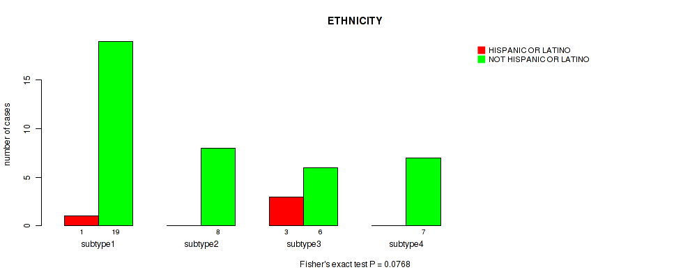
'Methylation CNMF subtypes' versus 'ETHNICITY'

P value = 0.0768 (Fisher's exact test), Q value = 0.43

Table S29. Clustering Approach #2: 'Methylation CNMF subtypes' versus Clinical Feature #10: 'ETHNICITY'

nPatients	HISPANIC OR LATINO	NOT HISPANIC OR LATINO
ALL	4	40
subtype1	1	19
subtype2	0	8
subtype3	3	6
subtype4	0	7

Figure S27. Get High-res Image Clustering Approach #2: 'Methylation CNMF subtypes' versus Clinical Feature #10: 'ETHNICITY'

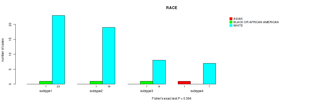
'Methylation CNMF subtypes' versus 'RACE'

P value = 0.364 (Fisher's exact test), Q value = 0.83

Table S30. Clustering Approach #2: 'Methylation CNMF subtypes' versus Clinical Feature #11: 'RACE'

nPatients	ASIAN	BLACK OR AFRICAN AMERICAN	WHITE
ALL	1	3	57
subtype1	0	1	23
subtype2	0	1	19
subtype3	0	1	8
subtype4	1	0	7

Figure S28. Get High-res Image Clustering Approach #2: 'Methylation CNMF subtypes' versus Clinical Feature #11: 'RACE'

'Methylation CNMF subtypes' versus 'RADIATION_THERAPY'

P value = 0.105 (Fisher's exact test), Q value = 0.46

Table S31. Clustering Approach #2: 'Methylation CNMF subtypes' versus Clinical Feature #12: 'RADIATION_THERAPY'

nPatients	NO	YES
ALL	43	52
subtype1	18	16
subtype2	13	20
subtype3	4	12
subtype4	8	4

Figure S29. Get High-res Image Clustering Approach #2: 'Methylation CNMF subtypes' versus Clinical Feature #12: 'RADIATION_THERAPY'

'Methylation CNMF subtypes' versus 'DIABETES'

P value = 0.0655 (Fisher's exact test), Q value = 0.42

Table S32. Clustering Approach #2: 'Methylation CNMF subtypes' versus Clinical Feature #13: 'DIABETES'

nPatients	NO	YES
ALL	68	27
subtype1	23	11
subtype2	24	9
subtype3	15	1
subtype4	6	6

Figure S30. Get High-res Image Clustering Approach #2: 'Methylation CNMF subtypes' versus Clinical Feature #13: 'DIABETES'

'Methylation CNMF subtypes' versus 'BMI'

P value = 0.0515 (Fisher's exact test), Q value = 0.42

Table S33. Clustering Approach #2: 'Methylation CNMF subtypes' versus Clinical Feature #14: 'BMI'

nPatients	NORMAL	OBESE	OVERWEIGHT	SEVERELY OBESE	UNDERWEIGHT
ALL	7	45	20	21	3
subtype1	3	12	7	10	3
subtype2	1	21	4	7	0
subtype3	3	5	7	1	0
subtype4	0	7	2	3	0

Figure S31. Get High-res Image Clustering Approach #2: 'Methylation CNMF subtypes' versus Clinical Feature #14: 'BMI'

'Methylation CNMF subtypes' versus 'NUMBER_PACK_YEARS_SMOKED'

P value = 0.153 (Kruskal-Wallis (anova)), Q value = 0.52

Table S34. Clustering Approach #2: 'Methylation CNMF subtypes' versus Clinical Feature #15: 'NUMBER_PACK_YEARS_SMOKED'

	nPatients	Mean (Std.Dev)
ALL	18	14.5 (11.9)
subtype1	7	18.8 (13.2)
subtype2	9	12.0 (11.0)
subtype4	2	10.5 (13.4)

Figure S32. Get High-res Image Clustering Approach #2: 'Methylation CNMF subtypes' versus Clinical Feature #15: 'NUMBER_PACK_YEARS_SMOKED'

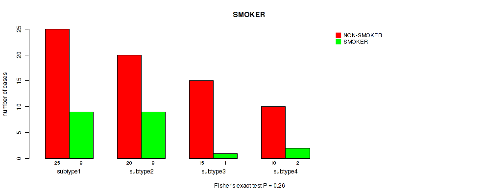
'Methylation CNMF subtypes' versus 'SMOKER'

P value = 0.26 (Fisher's exact test), Q value = 0.79

Table S35. Clustering Approach #2: 'Methylation CNMF subtypes' versus Clinical Feature #16: 'SMOKER'

nPatients	NON-SMOKER	SMOKER
ALL	70	21
subtype1	25	9
subtype2	20	9
subtype3	15	1
subtype4	10	2

Figure S33. Get High-res Image Clustering Approach #2: 'Methylation CNMF subtypes' versus Clinical Feature #16: 'SMOKER'

'Methylation CNMF subtypes' versus 'COUNTRY_OF_ORIGIN'

P value = 0.679 (Fisher's exact test), Q value = 0.91

Table S36. Clustering Approach #2: 'Methylation CNMF subtypes' versus Clinical Feature #17: 'COUNTRY_OF_ORIGIN'

nPatients	MEXICO	POLAND	UKRAINE	UNITED STATES
ALL	2	3	31	35
subtype1	1	2	9	16
subtype2	0	1	11	6
subtype3	1	0	7	8
subtype4	0	0	4	5

Figure S34. Get High-res Image Clustering Approach #2: 'Methylation CNMF subtypes' versus Clinical Feature #17: 'COUNTRY_OF_ORIGIN'

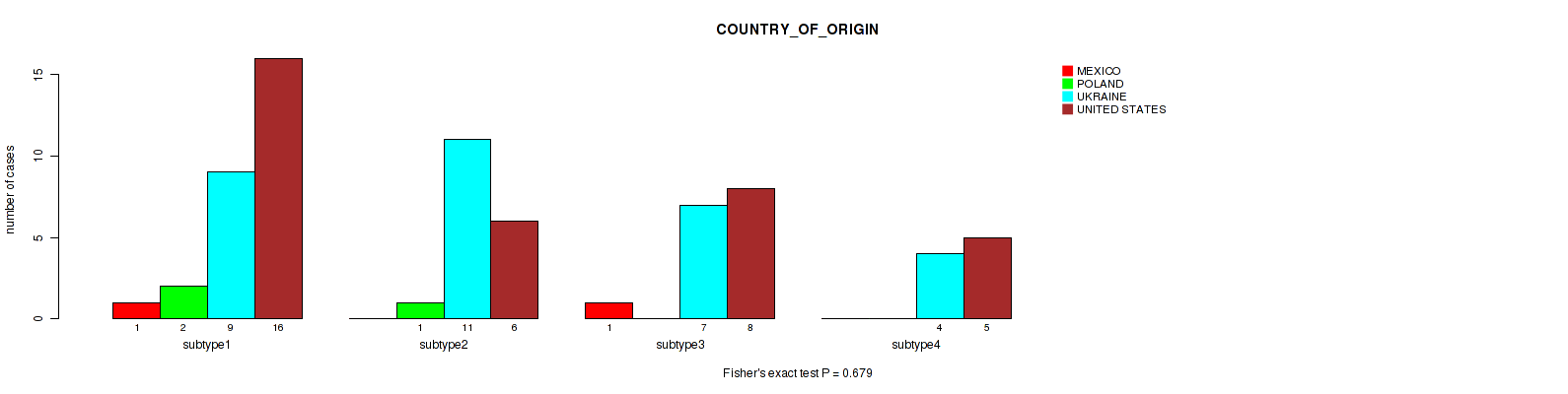
Clustering Approach #3: 'METHYLATION CHIERARCHICAL'

Table S37. Description of clustering approach #3: 'METHYLATION CHIERARCHICAL'

Cluster Labels	1	2	3	4	5	6	7
Number of samples	34	11	9	7	6	20	9

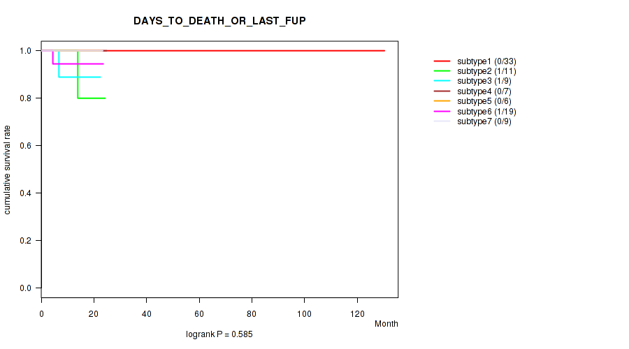
'METHYLATION CHIERARCHICAL' versus 'DAYS_TO_DEATH_OR_LAST_FUP'

P value = 0.585 (logrank test), Q value = 0.85

Table S38. Clustering Approach #3: 'METHYLATION CHIERARCHICAL' versus Clinical Feature #1: 'DAYS_TO_DEATH_OR_LAST_FUP'

	nPatients	nDeath	Duration Range (Median), Month
ALL	95	3	1.9 - 130.4 (11.6)
subtype1	33	0	6.1 - 130.4 (11.1)
subtype2	11	1	5.4 - 24.3 (13.1)
subtype3	9	1	6.7 - 22.4 (17.5)
subtype4	7	0	1.9 - 24.8 (22.6)
subtype5	6	0	10.4 - 22.9 (17.1)
subtype6	19	1	2.3 - 23.5 (9.6)
subtype7	9	0	8.2 - 23.3 (14.0)

Figure S35. Get High-res Image Clustering Approach #3: 'METHYLATION CHIERARCHICAL' versus Clinical Feature #1: 'DAYS_TO_DEATH_OR_LAST_FUP'

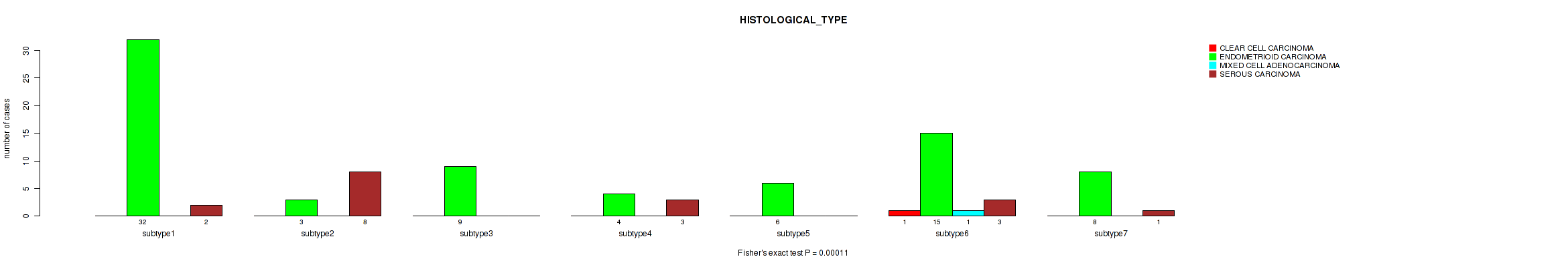
'METHYLATION CHIERARCHICAL' versus 'HISTOLOGICAL_TYPE'

P value = 0.00011 (Fisher's exact test), Q value = 0.0056

Table S39. Clustering Approach #3: 'METHYLATION CHIERARCHICAL' versus Clinical Feature #2: 'HISTOLOGICAL_TYPE'

nPatients	CLEAR CELL CARCINOMA	ENDOMETRIOID CARCINOMA	MIXED CELL ADENOCARCINOMA	SEROUS CARCINOMA
ALL	1	77	1	17
subtype1	0	32	0	2
subtype2	0	3	0	8
subtype3	0	9	0	0
subtype4	0	4	0	3
subtype5	0	6	0	0
subtype6	1	15	1	3
subtype7	0	8	0	1

Figure S36. Get High-res Image Clustering Approach #3: 'METHYLATION CHIERARCHICAL' versus Clinical Feature #2: 'HISTOLOGICAL_TYPE'

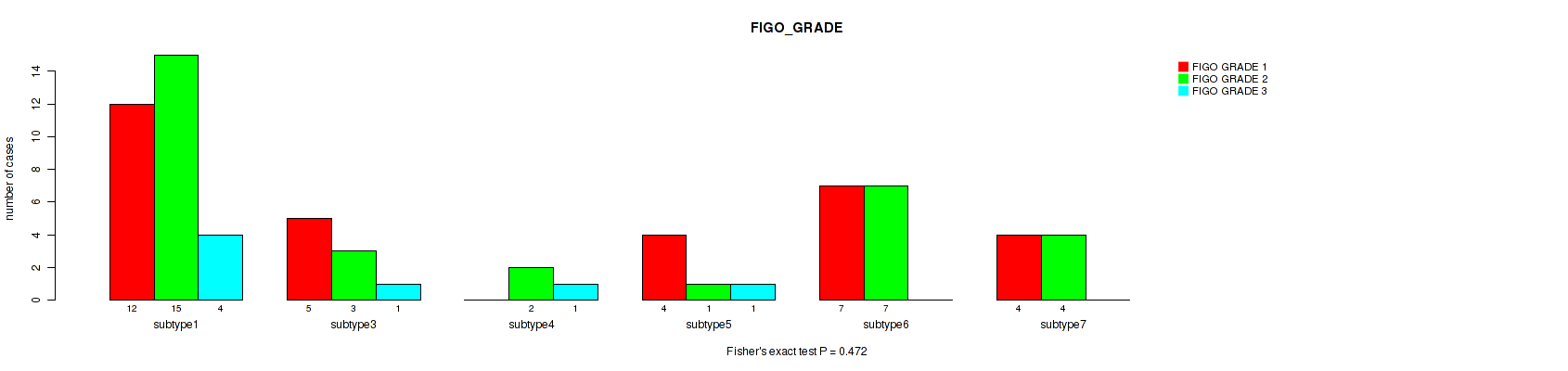
'METHYLATION CHIERARCHICAL' versus 'FIGO_GRADE'

P value = 0.472 (Fisher's exact test), Q value = 0.83

Table S40. Clustering Approach #3: 'METHYLATION CHIERARCHICAL' versus Clinical Feature #3: 'FIGO_GRADE'

nPatients	FIGO GRADE 1	FIGO GRADE 2	FIGO GRADE 3
ALL	32	34	7
subtype1	12	15	4
subtype2	0	2	0
subtype3	5	3	1
subtype4	0	2	1
subtype5	4	1	1
subtype6	7	7	0
subtype7	4	4	0

Figure S37. Get High-res Image Clustering Approach #3: 'METHYLATION CHIERARCHICAL' versus Clinical Feature #3: 'FIGO_GRADE'

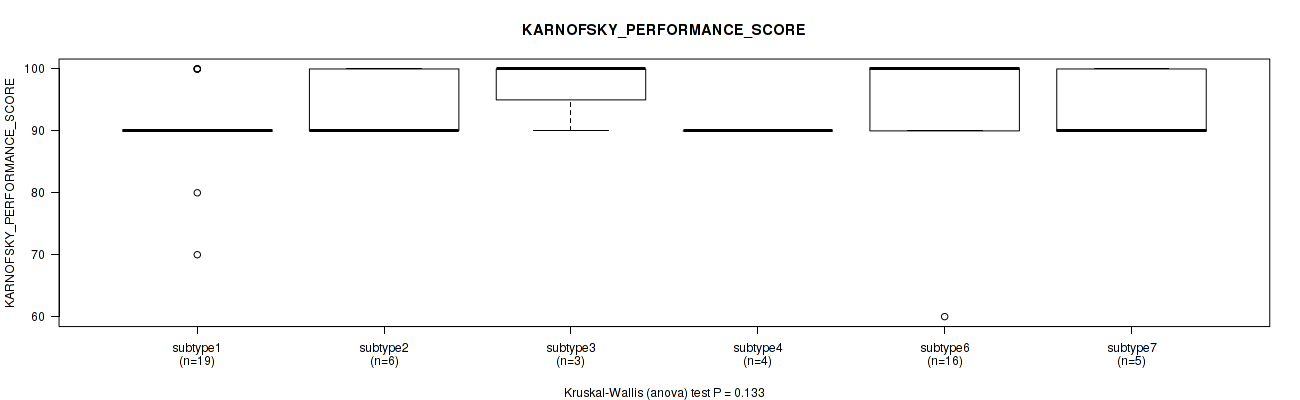
'METHYLATION CHIERARCHICAL' versus 'KARNOFSKY_PERFORMANCE_SCORE'

P value = 0.133 (Kruskal-Wallis (anova)), Q value = 0.52

Table S41. Clustering Approach #3: 'METHYLATION CHIERARCHICAL' versus Clinical Feature #4: 'KARNOFSKY_PERFORMANCE_SCORE'

	nPatients	Mean (Std.Dev)
ALL	55	92.7 (7.6)
subtype1	19	90.5 (7.1)
subtype2	6	93.3 (5.2)
subtype3	3	96.7 (5.8)
subtype4	4	90.0 (0.0)
subtype5	2	95.0 (7.1)
subtype6	16	94.4 (10.3)
subtype7	5	94.0 (5.5)

Figure S38. Get High-res Image Clustering Approach #3: 'METHYLATION CHIERARCHICAL' versus Clinical Feature #4: 'KARNOFSKY_PERFORMANCE_SCORE'

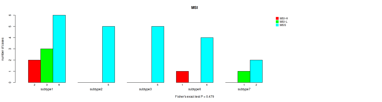
'METHYLATION CHIERARCHICAL' versus 'MSI'

P value = 0.479 (Fisher's exact test), Q value = 0.83

Table S42. Clustering Approach #3: 'METHYLATION CHIERARCHICAL' versus Clinical Feature #5: 'MSI'

nPatients	MSI-H	MSI-L	MSS
ALL	4	5	23
subtype1	2	3	6
subtype2	0	0	5
subtype3	0	0	5
subtype4	0	0	1
subtype5	1	1	0
subtype6	1	0	4
subtype7	0	1	2

Figure S39. Get High-res Image Clustering Approach #3: 'METHYLATION CHIERARCHICAL' versus Clinical Feature #5: 'MSI'

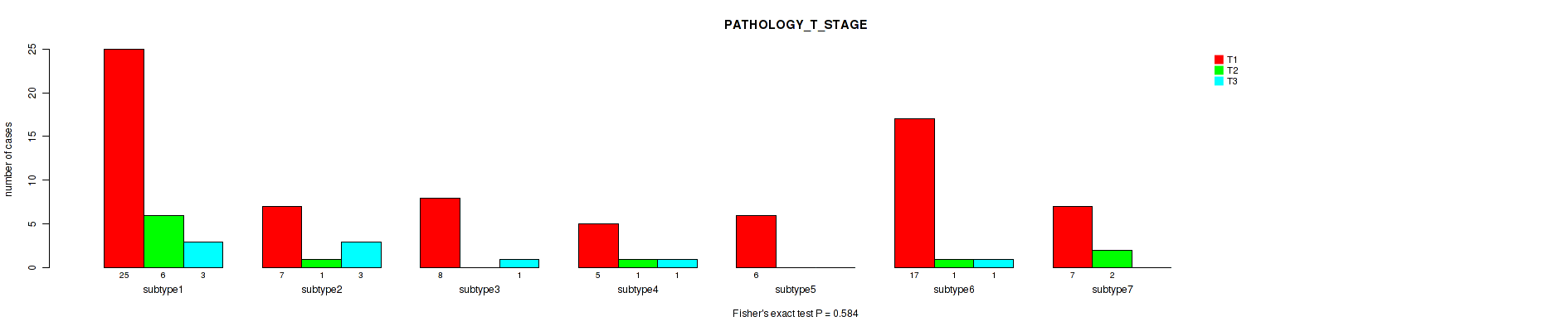
'METHYLATION CHIERARCHICAL' versus 'PATHOLOGY_T_STAGE'

P value = 0.584 (Kruskal-Wallis (anova)), Q value = 0.85

Table S43. Clustering Approach #3: 'METHYLATION CHIERARCHICAL' versus Clinical Feature #6: 'PATHOLOGY_T_STAGE'

	T1	T2	T3
ALL	75	11	9
subtype1	25	6	3
subtype2	7	1	3
subtype3	8	0	1
subtype4	5	1	1
subtype5	6	0	0
subtype6	17	1	1
subtype7	7	2	0

Figure S40. Get High-res Image Clustering Approach #3: 'METHYLATION CHIERARCHICAL' versus Clinical Feature #6: 'PATHOLOGY_T_STAGE'

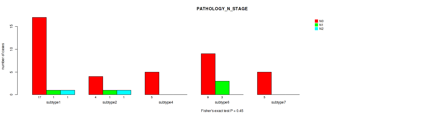
'METHYLATION CHIERARCHICAL' versus 'PATHOLOGY_N_STAGE'

P value = 0.45 (Kruskal-Wallis (anova)), Q value = 0.83

Table S44. Clustering Approach #3: 'METHYLATION CHIERARCHICAL' versus Clinical Feature #7: 'PATHOLOGY_N_STAGE'

	N0	N1	N2
ALL	44	5	2
subtype1	17	1	1
subtype2	4	1	1
subtype3	2	0	0
subtype4	5	0	0
subtype5	2	0	0
subtype6	9	3	0
subtype7	5	0	0

Figure S41. Get High-res Image Clustering Approach #3: 'METHYLATION CHIERARCHICAL' versus Clinical Feature #7: 'PATHOLOGY_N_STAGE'

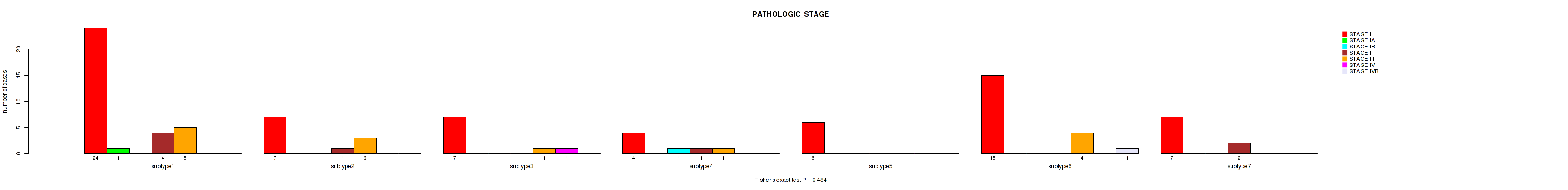
'METHYLATION CHIERARCHICAL' versus 'PATHOLOGIC_STAGE'

P value = 0.484 (Fisher's exact test), Q value = 0.83

Table S45. Clustering Approach #3: 'METHYLATION CHIERARCHICAL' versus Clinical Feature #8: 'PATHOLOGIC_STAGE'

nPatients	STAGE I	STAGE IA	STAGE IB	STAGE II	STAGE III	STAGE IV	STAGE IVB
ALL	70	1	1	8	14	1	1
subtype1	24	1	0	4	5	0	0
subtype2	7	0	0	1	3	0	0
subtype3	7	0	0	0	1	1	0
subtype4	4	0	1	1	1	0	0
subtype5	6	0	0	0	0	0	0
subtype6	15	0	0	0	4	0	1
subtype7	7	0	0	2	0	0	0

Figure S42. Get High-res Image Clustering Approach #3: 'METHYLATION CHIERARCHICAL' versus Clinical Feature #8: 'PATHOLOGIC_STAGE'

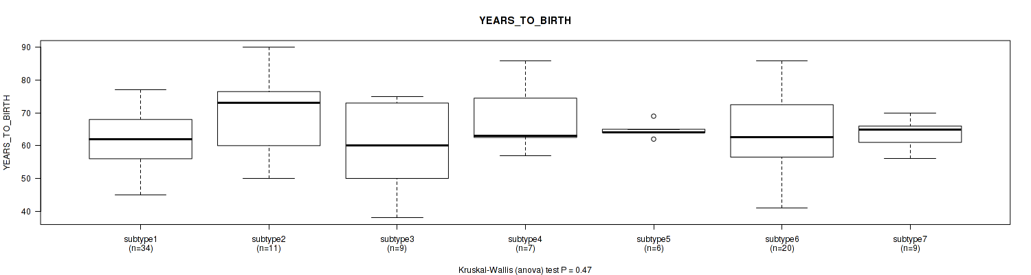
'METHYLATION CHIERARCHICAL' versus 'YEARS_TO_BIRTH'

P value = 0.47 (Kruskal-Wallis (anova)), Q value = 0.83

Table S46. Clustering Approach #3: 'METHYLATION CHIERARCHICAL' versus Clinical Feature #9: 'YEARS_TO_BIRTH'

	nPatients	Mean (Std.Dev)
ALL	96	63.5 (10.2)
subtype1	34	61.5 (8.2)
subtype2	11	69.7 (12.0)
subtype3	9	59.6 (13.4)
subtype4	7	68.6 (11.8)
subtype5	6	64.7 (2.3)
subtype6	20	62.8 (12.2)
subtype7	9	63.9 (4.5)

Figure S43. Get High-res Image Clustering Approach #3: 'METHYLATION CHIERARCHICAL' versus Clinical Feature #9: 'YEARS_TO_BIRTH'

'METHYLATION CHIERARCHICAL' versus 'ETHNICITY'

P value = 0.844 (Fisher's exact test), Q value = 0.91

Table S47. Clustering Approach #3: 'METHYLATION CHIERARCHICAL' versus Clinical Feature #10: 'ETHNICITY'

nPatients	HISPANIC OR LATINO	NOT HISPANIC OR LATINO
ALL	4	40
subtype1	3	14
subtype2	1	4
subtype3	0	7
subtype4	0	3
subtype5	0	4
subtype6	0	4
subtype7	0	4

Figure S44. Get High-res Image Clustering Approach #3: 'METHYLATION CHIERARCHICAL' versus Clinical Feature #10: 'ETHNICITY'

'METHYLATION CHIERARCHICAL' versus 'RACE'

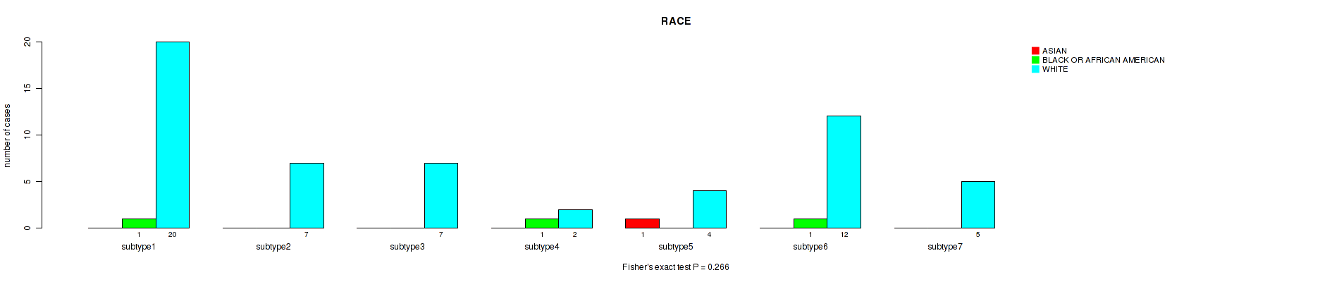
P value = 0.266 (Fisher's exact test), Q value = 0.79

Table S48. Clustering Approach #3: 'METHYLATION CHIERARCHICAL' versus Clinical Feature #11: 'RACE'

nPatients	ASIAN	BLACK OR AFRICAN AMERICAN	WHITE
ALL	1	3	57
subtype1	0	1	20
subtype2	0	0	7
subtype3	0	0	7
subtype4	0	1	2
subtype5	1	0	4
subtype6	0	1	12
subtype7	0	0	5

Figure S45. Get High-res Image Clustering Approach #3: 'METHYLATION CHIERARCHICAL' versus Clinical Feature #11: 'RACE'

'METHYLATION CHIERARCHICAL' versus 'RADIATION_THERAPY'

P value = 0.0145 (Fisher's exact test), Q value = 0.25

Table S49. Clustering Approach #3: 'METHYLATION CHIERARCHICAL' versus Clinical Feature #12: 'RADIATION_THERAPY'

nPatients	NO	YES
ALL	43	52
subtype1	12	21
subtype2	5	6
subtype3	9	0
subtype4	2	5
subtype5	4	2
subtype6	8	12
subtype7	3	6

Figure S46. Get High-res Image Clustering Approach #3: 'METHYLATION CHIERARCHICAL' versus Clinical Feature #12: 'RADIATION_THERAPY'

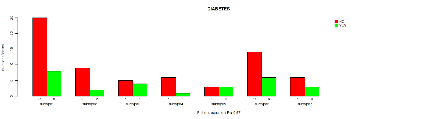
'METHYLATION CHIERARCHICAL' versus 'DIABETES'

P value = 0.67 (Fisher's exact test), Q value = 0.91

Table S50. Clustering Approach #3: 'METHYLATION CHIERARCHICAL' versus Clinical Feature #13: 'DIABETES'

nPatients	NO	YES
ALL	68	27
subtype1	25	8
subtype2	9	2
subtype3	5	4
subtype4	6	1
subtype5	3	3
subtype6	14	6
subtype7	6	3

Figure S47. Get High-res Image Clustering Approach #3: 'METHYLATION CHIERARCHICAL' versus Clinical Feature #13: 'DIABETES'

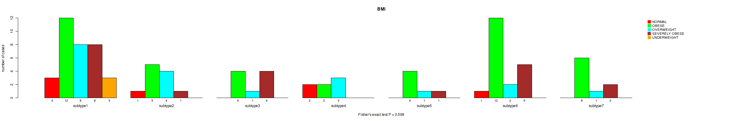
'METHYLATION CHIERARCHICAL' versus 'BMI'

P value = 0.598 (Fisher's exact test), Q value = 0.85

Table S51. Clustering Approach #3: 'METHYLATION CHIERARCHICAL' versus Clinical Feature #14: 'BMI'

nPatients	NORMAL	OBESE	OVERWEIGHT	SEVERELY OBESE	UNDERWEIGHT
ALL	7	45	20	21	3
subtype1	3	12	8	8	3
subtype2	1	5	4	1	0
subtype3	0	4	1	4	0
subtype4	2	2	3	0	0
subtype5	0	4	1	1	0
subtype6	1	12	2	5	0
subtype7	0	6	1	2	0

Figure S48. Get High-res Image Clustering Approach #3: 'METHYLATION CHIERARCHICAL' versus Clinical Feature #14: 'BMI'

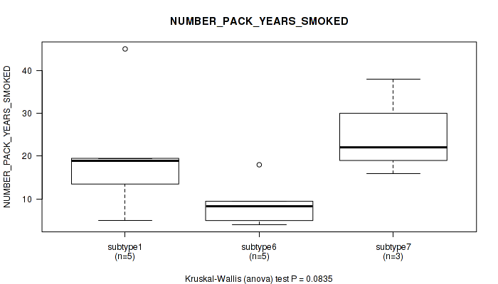
'METHYLATION CHIERARCHICAL' versus 'NUMBER_PACK_YEARS_SMOKED'

P value = 0.0835 (Kruskal-Wallis (anova)), Q value = 0.43

Table S52. Clustering Approach #3: 'METHYLATION CHIERARCHICAL' versus Clinical Feature #15: 'NUMBER_PACK_YEARS_SMOKED'

	nPatients	Mean (Std.Dev)
ALL	18	14.5 (11.9)
subtype1	5	20.4 (14.9)
subtype2	2	4.7 (2.3)
subtype3	2	13.8 (8.8)
subtype5	1	1.0 (NA)
subtype6	5	9.0 (5.5)
subtype7	3	25.3 (11.4)

Figure S49. Get High-res Image Clustering Approach #3: 'METHYLATION CHIERARCHICAL' versus Clinical Feature #15: 'NUMBER_PACK_YEARS_SMOKED'

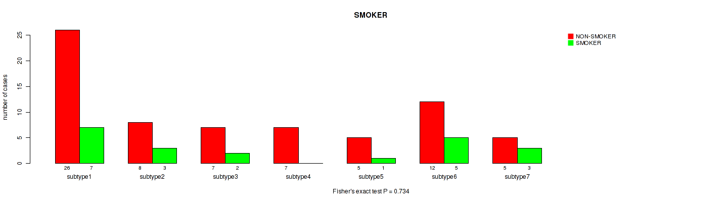
'METHYLATION CHIERARCHICAL' versus 'SMOKER'

P value = 0.734 (Fisher's exact test), Q value = 0.91

Table S53. Clustering Approach #3: 'METHYLATION CHIERARCHICAL' versus Clinical Feature #16: 'SMOKER'

nPatients	NON-SMOKER	SMOKER
ALL	70	21
subtype1	26	7
subtype2	8	3
subtype3	7	2
subtype4	7	0
subtype5	5	1
subtype6	12	5
subtype7	5	3

Figure S50. Get High-res Image Clustering Approach #3: 'METHYLATION CHIERARCHICAL' versus Clinical Feature #16: 'SMOKER'

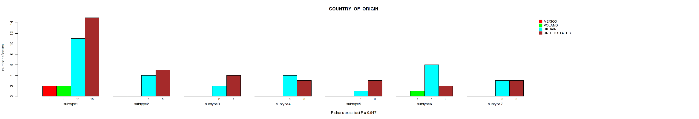
'METHYLATION CHIERARCHICAL' versus 'COUNTRY_OF_ORIGIN'

P value = 0.947 (Fisher's exact test), Q value = 0.97

Table S54. Clustering Approach #3: 'METHYLATION CHIERARCHICAL' versus Clinical Feature #17: 'COUNTRY_OF_ORIGIN'

nPatients	MEXICO	POLAND	UKRAINE	UNITED STATES
ALL	2	3	31	35
subtype1	2	2	11	15
subtype2	0	0	4	5
subtype3	0	0	2	4
subtype4	0	0	4	3
subtype5	0	0	1	3
subtype6	0	1	6	2
subtype7	0	0	3	3

Figure S51. Get High-res Image Clustering Approach #3: 'METHYLATION CHIERARCHICAL' versus Clinical Feature #17: 'COUNTRY_OF_ORIGIN'

Methods & Data

Input

Cluster data file = /cromwell_root/fc-8b2df640-93e1-40a2-b735-5b7a14ef6398/10d02b45-07ea-40cc-ac82-013e5f89ebb2/aggregate_clusters_workflow/b0f8dcb2-0993-4424-ad42-552c0bd1a2d5/call-aggregate_clusters/CPTAC3-UCEC-TP.mergedcluster.txt
Clinical data file = /cromwell_root/fc-8b2df640-93e1-40a2-b735-5b7a14ef6398/f48b4003-eaf7-47c4-8ca4-0ddbd4729902/normalize_clinical_cptac/0ea0fb0d-64a4-4204-8245-a79f52e6cd0a/call-normalize_clinical_cptac_task_1/CPTAC3-UCEC-TP.clin.merged.picked.txt
Number of patients = 100
Number of clustering approaches = 3
Number of selected clinical features = 17
Exclude small clusters that include fewer than K patients, K = 3

Clustering approaches

Consensus hierarchical clustering

Resampling-based clustering method (Monti et al. 2003)

CNMF clustering

consensus non-negative matrix factorization clustering approach (Brunet et al. 2004)

Survival analysis

For survival clinical features, the Kaplan-Meier survival curves of tumors with and without gene mutations were plotted and the statistical significance P values were estimated by logrank test (Bland and Altman 2004) using the 'survdiff' function in R

Fisher's exact test

For binary clinical features, two-tailed Fisher's exact tests (Fisher 1922) were used to estimate the P values using the 'fisher.test' function in R

Q value calculation

For multiple hypothesis correction, Q value is the False Discovery Rate (FDR) analogue of the P value (Benjamini and Hochberg 1995), defined as the minimum FDR at which the test may be called significant. We used the 'Benjamini and Hochberg' method of 'p.adjust' function in R to convert P values into Q values.

References

[1] Monti et al., Consensus Clustering: A Resampling-Based Method for Class Discovery and Visualization of Gene Expression Microarray Data, Machine Learning 52(1):91-118 (2003)

[2] Brunet et al., Metagenes and molecular pattern discovery using matrix factorization, PNAS 101(12):4164-9 (2004)

[3] Bland and Altman, Statistics notes: The logrank test, BMJ 328(7447):1073 (2004)

[4] Fisher, R.A., On the interpretation of chi-square from contingency tables, and the calculation of P, Journal of the Royal Statistical Society 85(1):87-94 (1922)

[5] Benjamini and Hochberg, Controlling the false discovery rate: a practical and powerful approach to multiple testing, Journal of the Royal Statistical Society Series B 59:289-300 (1995)

Made with Nozzle